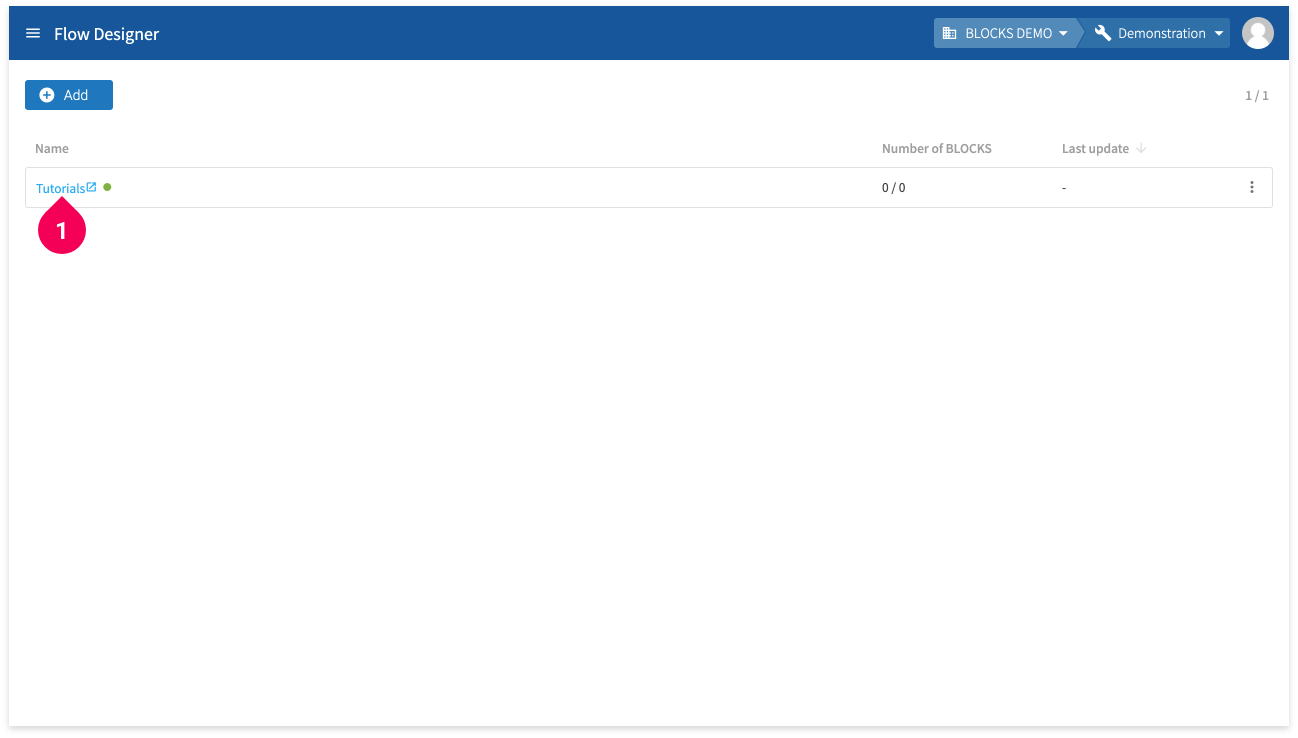
Demand forecasting with the regression model
Introduction
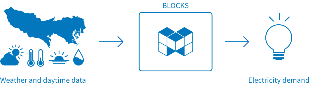
This tutorial will demonstrate how to use a deep learning-based regression model in BLOCKS. The regression model tries to determine the relationship between various input features and results variable (called the “label”). This model is often used to predict sales, customer numbers, and the like.
For the example in this tutorial, we’ll create a regression model using BLOCKS that uses input features for the weather and daytime minutes in the Tokyo region to predict for electricity demand.
General overview
This tutorial will show how to create a machine learning system in BLOCKS using the DataEditor and Flow Designer services. The basic steps will be as follows:
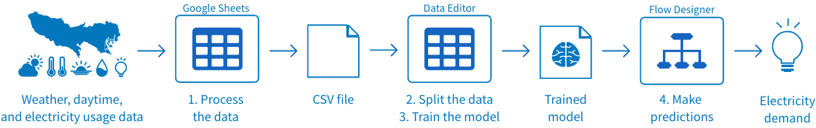
- Prepare the initial data in Google Sheets and download it as a CSV file.
- Upload the CSV file into the DataEditor and split it into training data and testing data.
- Run a training from the DataEditor:
BLOCKS will “learn” the relationship between the input features (weather/daytime minutes data) and the label (electricity usage).
The results that we get from the training are called a model or trained model. - Make electricity demand predictions from a Flow Designer.
Testing a regression model
We’ll do the following to train and use a regression model to predict Tokyo electricity demand:
- Prepare weather, daytime minutes, and electricity usage data for the Tokyo region as a CSV file.
- Use the DataEditor to split the data into training data and testing data.
- Train the model in the DataEditor.
- Prepare a Flow Designer.
- Create a processing flow for making predictions.
- Execute the flow.
- Check the results of the prediction in the DataEditor.
Good, properly formatted data is essential to machine learning and makes it possible to train models and make predictions. As such, the first step will be to gather and process our data to prepare it for use in machine learning.
We recommend using Google Chrome for this tutorial. BLOCKS also supports Firefox, but some steps in this tutorial may be slightly different if you aren’t using Google Chrome.
Preparing the data as a CSV file
The first step is to prepare the data we’ll use to train and test our regression model. We’ll prepare the initial data as a CSV file (UTF-8, without BOM).
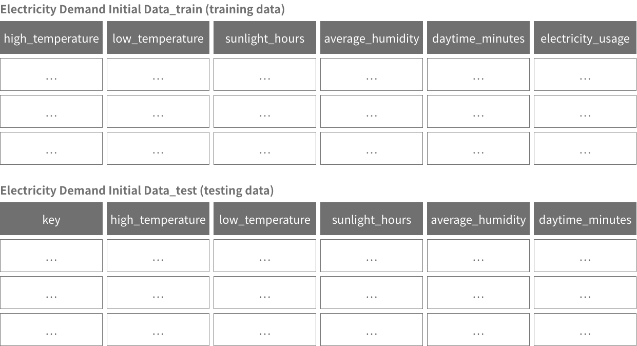
The training data will consist of the following information for the Tokyo region:
- High temperature
- Low temperature
- Sunlight hours
- Average humidity
- Daytime minutes
- Electricity usage
During the training, BLOCKS will “learn” the relationship that the weather/daytime minutes data has on electricity usage.
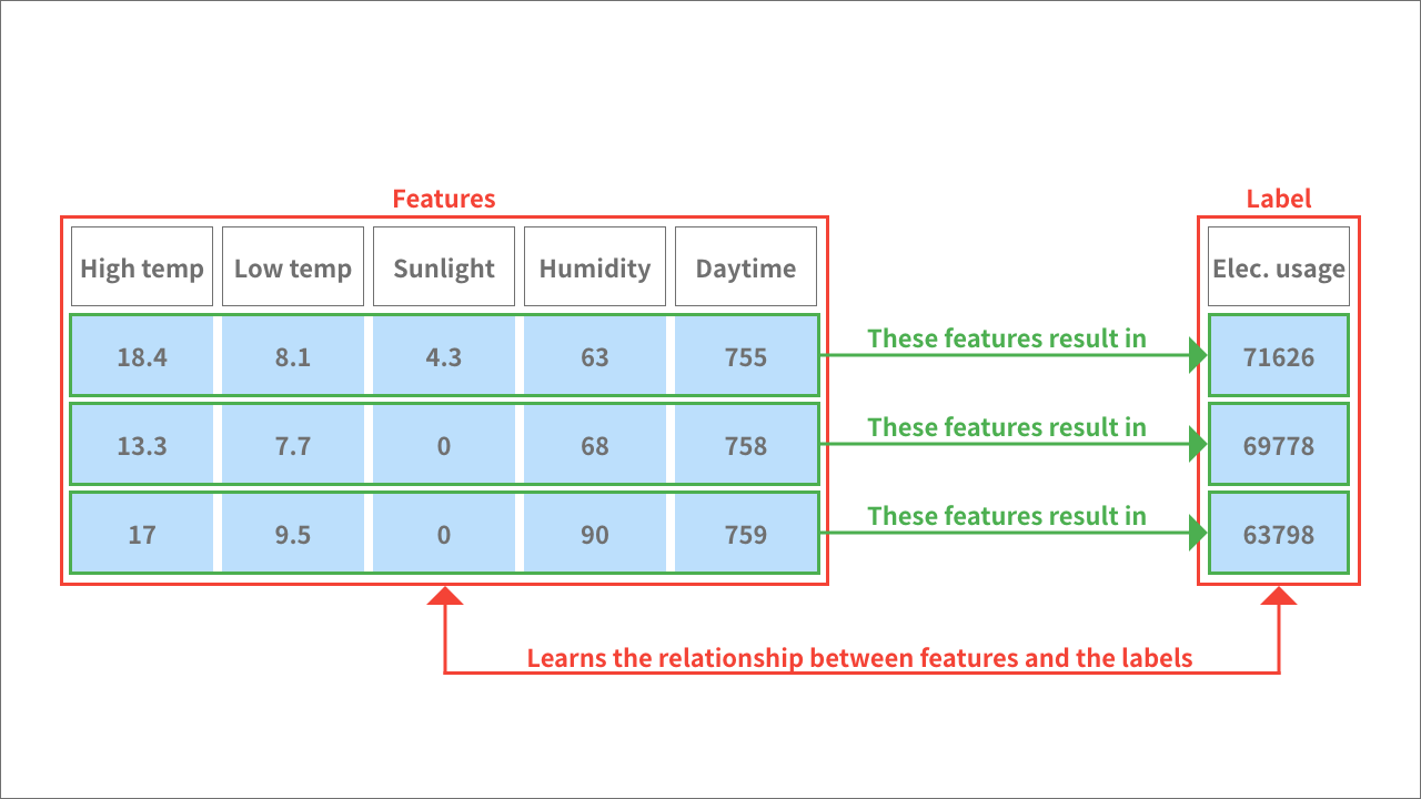
We refer to the input variables (high temp, low temp, sunlight hours, average humidity, and daytime minutes) as features. We refer to the dependent variable (electricity usage) as the label or results variable.
During the testing step, we’ll use feature data not used to train the model to predict electricity usage.
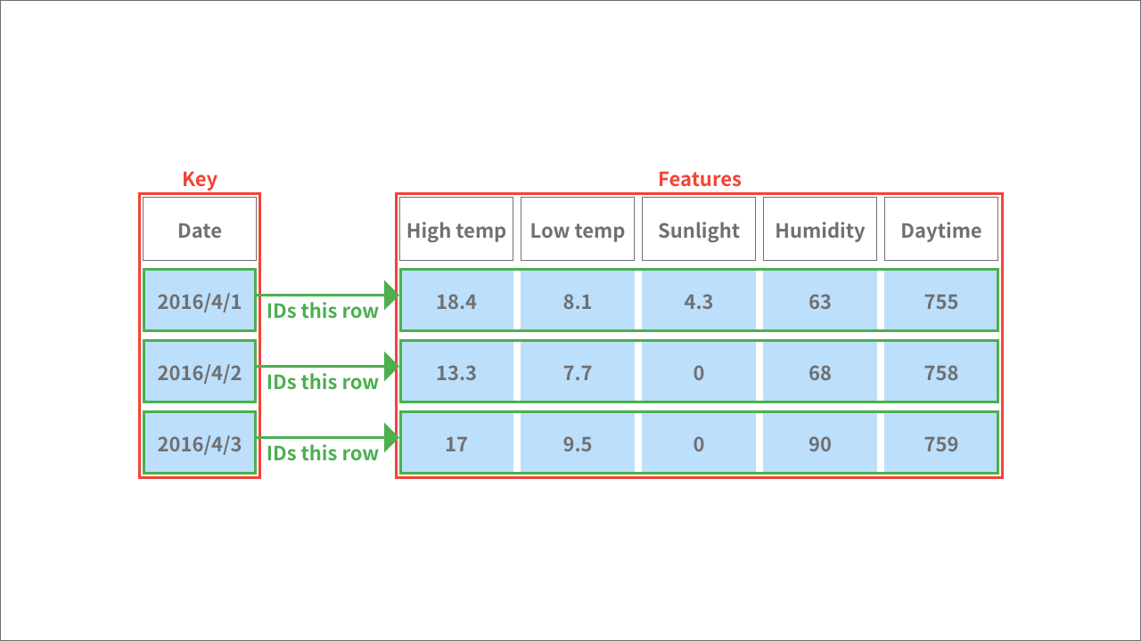
The data for testing the model should contain a column named key and the feature data. The key column contains values to identify each example (1 row) of features. Each value within the key column must be unique. In this example, we’ll use dates as our keys.
The initial data for this tutorial comes from the following sources:
- High temperature, low temperature, sunlight hours, and average humidity data: Japan Meteorological Agency open_in_new
- Daytime minutes data:National Astronomical Observatory of Japan open_in_new
- Electricity usage data: Tokyo Electric Power Company Holdings (TEPCO)open_in_new
info_outline The National Astronomical Observatory of Japan calculates daytime as the number of minutes between sunrise and sunset.
The time period for the data is shown in the following chart:
| Data type | Time period |
|---|---|
| Training data | January 1, 2016 through November 30, 2018 (2 years, 11 months). |
| Testing data | December 1, 2018 through December 31, 2018 (1 month). |
info_outline In an actual business use case, you would likely want to predict for future dates. However, this tutorial will demonstrate the testing step you would take before using your model in a business scenario. When testing a model, you predict for past data that wasn't used to train the model. By doing this, you can compare the results of the prediction with the actual data to evaluate the usefulness of the model.
We’ve the feature data you’ll need for this tutorial as a CSV file that you can download from the following link:
| Data | Explanation |
|---|---|
| cloud_download Sample weather data(weather_daytimeminutes.csv) |
A CSV file containing weather data from the Japan Meteorological Agency and daytime minutes data from the National Astronomical Observatory of Japan. It contains data for the Tokyo, Japan region for the dates January 1, 2016 through December 31, 2018.
Click the link in the left column to download the feature data. warning The Japan Meteorological Agency and National Astronomical Observatory of Japan assume no responsibility for any activity that uses this data. |
For the electricity demand data, you’ll need to download it directly from this TEPCO open_in_new page by doing the following:

- Right-click 2016.
- Click Save Link As....
- Select where to save the file and click Save.
Repeat these steps for the 2017 and 2018 links.
Once you’ve finished downloading all of the data, you’ll need to combine it with the feature data into one file that can be used in BLOCKS.
There are various ways to process the data and prepare it for use in machine learning, but this tutorial will follow the steps outlined in the image below. First, we’ll use Google Sheets to combine the feature and label data into one table and then download it as a CSV file. Next, we’ll upload that file into the DataEditor, cleanse the data, and split it into separate data for training and testing the model.
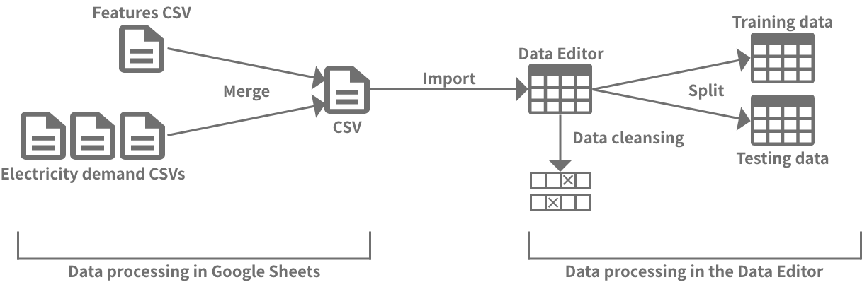
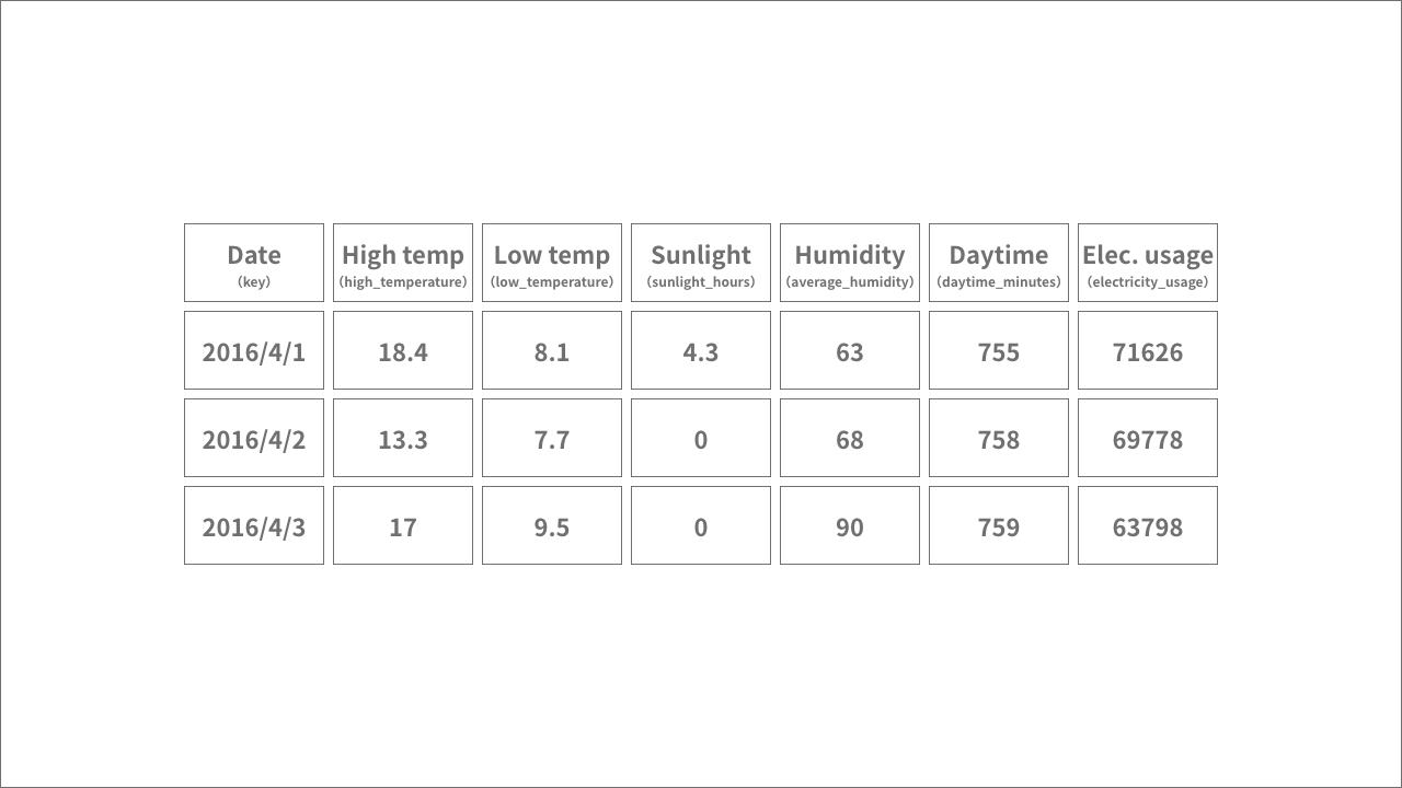
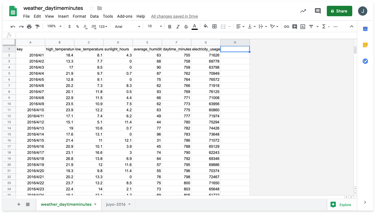
We’ll combine all of our feature and label data into one table in Google Sheets formatted as shown in the following chart. Note that the headers (actual headers are shown in parentheses) can only contain numbers, letters, or underscores (_).
(Click to enlarge image.)
info_outline The dates are not one of the features we’ll use to train the model, but they will be necessary when we test and evaluate it. We’ll use the dates in the testing data as the key column to identify each date’s example of data. This column must be named key.
To prepare the CSV file that we will upload to BLOCKS, open the weather_daytimeminutes.csv file in Google Sheets open_in_new.
Add the electricity usage data to a new sheet by doing the following:
- Click File.
- Click Import.
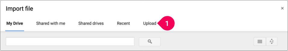
- Click Upload.
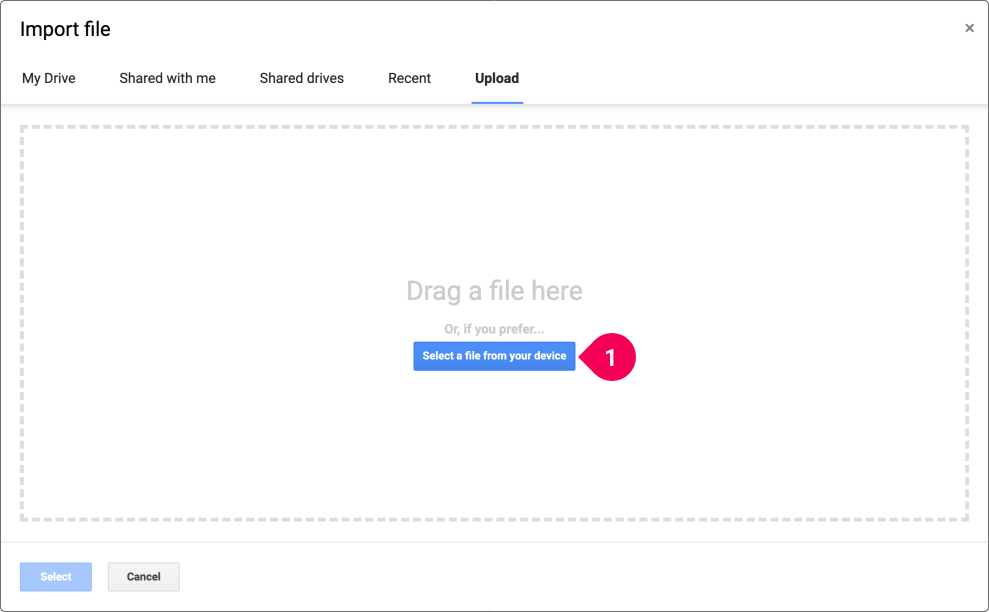
- Click Select a file from your device.
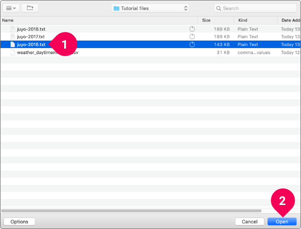
- Select the juyo-2016 file you downloaded.
- Click Open.

- Click the Insert new sheet(s).
- Click Import data.
Repeat this process for the 2017 and 2018 files, but do the following on the Import file section:
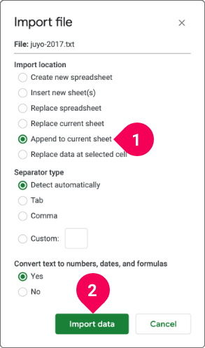
- Click Append to current sheet.
- Click Import data.
All of the electricity demand data should now be imported into the juyo-2016 sheet. However, each file contained header rows, so delete these from each year’s data by doing the following:
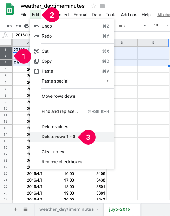
- Select rows 1–3.
- Click Edit.
- Click Delete rows 1–3.
The next header rows to delete are on rows 6601–6603. You can jump to these rows quickly by doing the following:
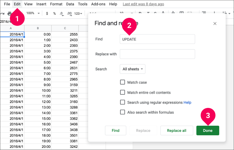
- Click Edit and select Find and replace.
- Enter UPDATE in the Find field.
- Click Done.
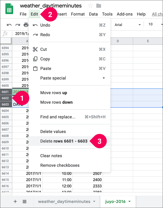
- Select rows 6601–6603.
- Click Edit.
- Click Delete rows 6601–6603.
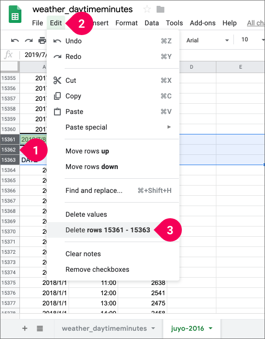
Repeat the previous steps to find the next set of header rows and do the following:
- Select rows 15361–15363.
- Click Edit.
- Click Delete rows 15361–15363.
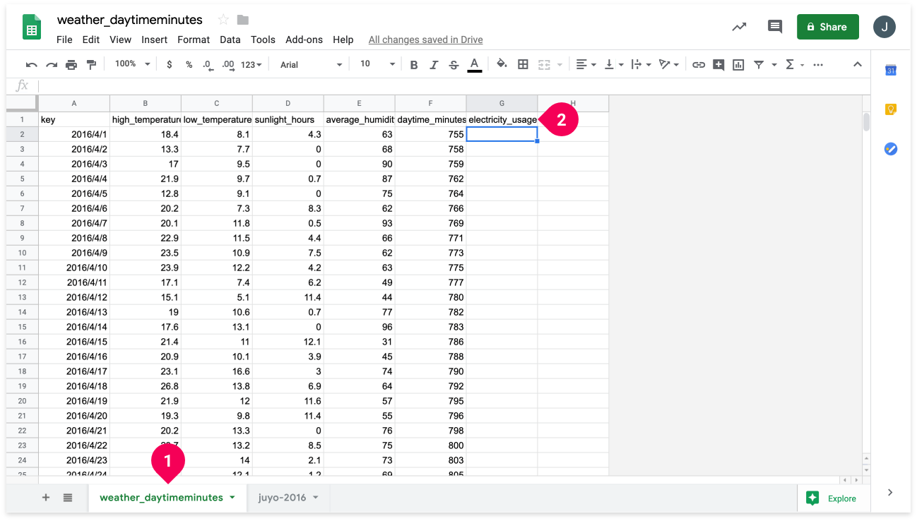
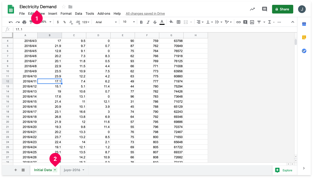
- Click the weather_daytimeminutes tab.
- Enter electricity_usage into cell G1.
- Enter
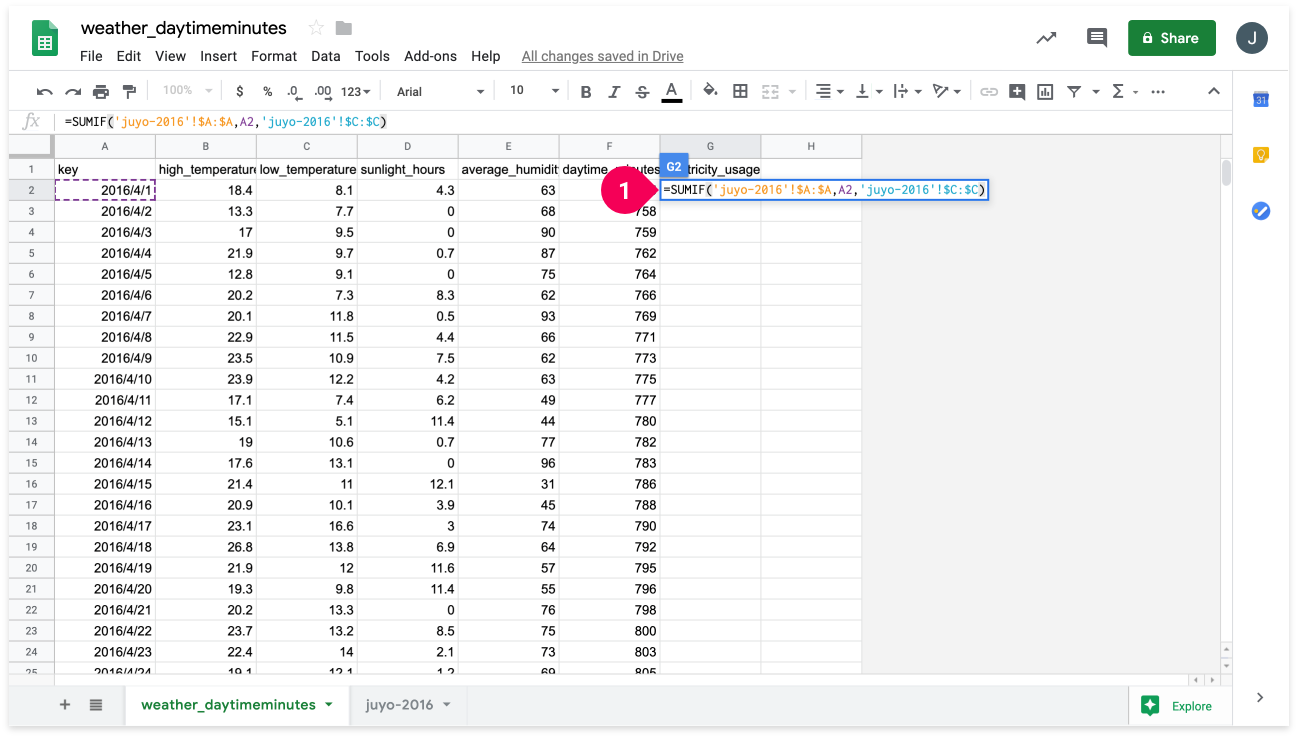
=SUMIF('juyo-2016'!$A:$A,A2,'juyo-2016'!$C:$C)into cell G2.
This will calculate the amount of electricity used on April 1, 2016 and enter it into cell G2 as shown in the following image:
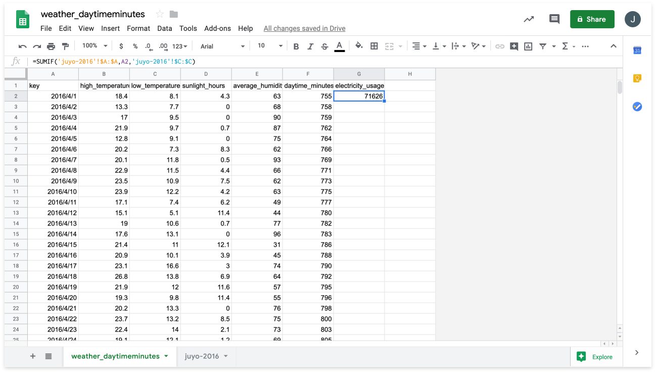
You can use this same formula to calculate electricity usage for the rest of the dates by doing the following:
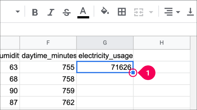
- Select cell G2 and double click the square in its bottom-right corner.
This will fill in the rest of the electricity_usage column with data for each date as shown in the following image:
Now the the data is ready, we’ll rename the sheet and file to make it more easily identifiable, then download it as a CSV file. First, do the following:
- Click weather_daytimeminutes and rename the file to Electricity Demand.
- Click the triangle icon on the right side of the weather_daytimeminutes tab, select Rename, then rename the tab to Initial Data.
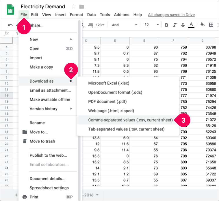
- Click File.
- Click Download as.
- Click Comma-separated values (.csv, current sheet).
This will download the data to your computer as Electricity Demand - Initial Data.csv.
You’re now done using Google Sheets for the initial data preparation. In the next section, we’ll import the CSV file into the DataEditor in BLOCKS.
Splitting the data in the DataEditor
Now that the initial data is ready, we need to cleanse it (remove missing values) and split it into separate data for training and testing the model. We can do all of this in the DataEditor in BLOCKS.
First, sign in to BLOCKS if you haven’t already. Then, do the following:
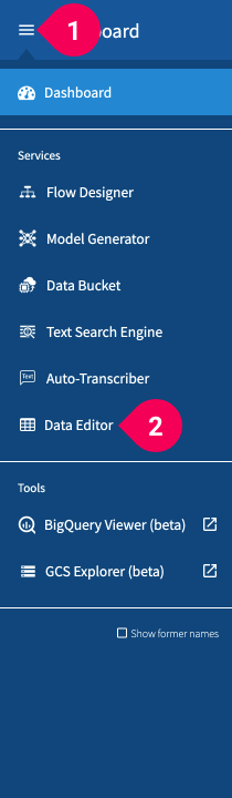
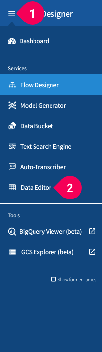
- Click the menu icon (menu) in the global navigation bar.
- Click DataEditor.
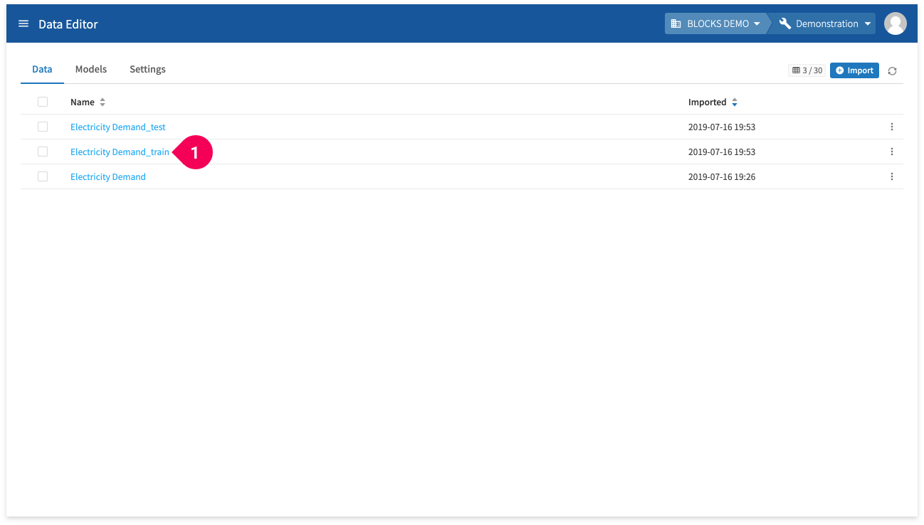
Import the data CSV file into the DataEditor by doing the following:
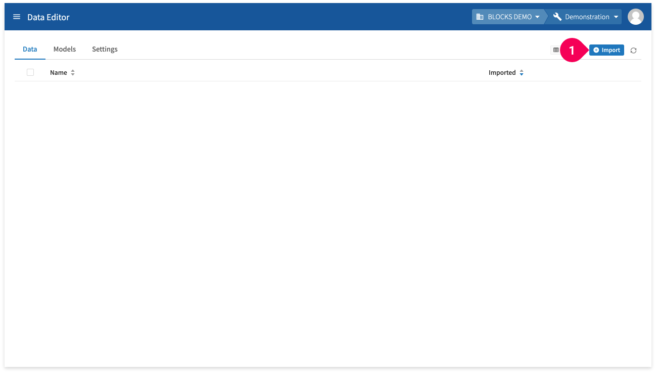
Click Import.
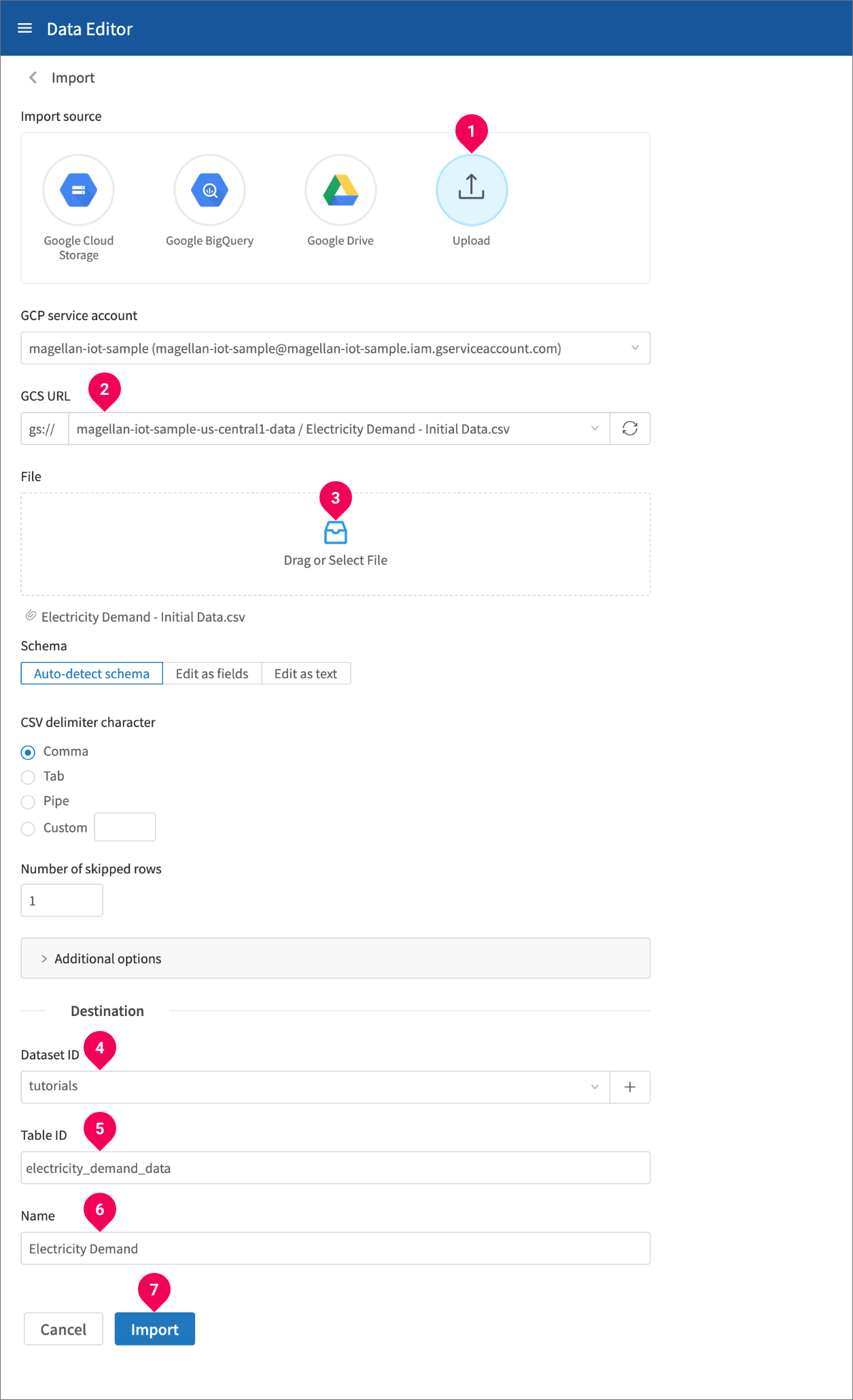
- Click Upload.
- Select the Google Cloud Storage (GCS) location to upload the file into. We’ll use a bucket that ends with -data.
- Drag and drop the Electricity Demand - Initial Data.csv file into the field or click and select the file.
- Select the dataset that will store the data or click + to create a new dataset. We’ll use a dataset called
tutorials. - Enter a name for the table. We’ll name our table
electricity_demand_data. - Enter a name that will identify the data in the DataEditor. We’ll use the name
Electricity Demand. - Click Import.
info_outline The DataEditor is a tool for visualizing and processing data that is stored in BigQuery. You don’t need to have any specialized knowledge of BigQuery to use the DataEditor. However, you do need to specify the BigQuery dataset and table that will store your data. If you are familiar with spreadsheet software, a BigQuery dataset could be compared to a workbook, and a BigQuery table to a single sheet.
Click Open.
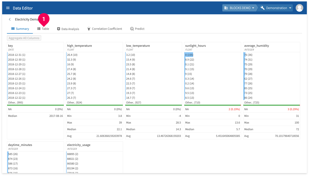
- Click Table.
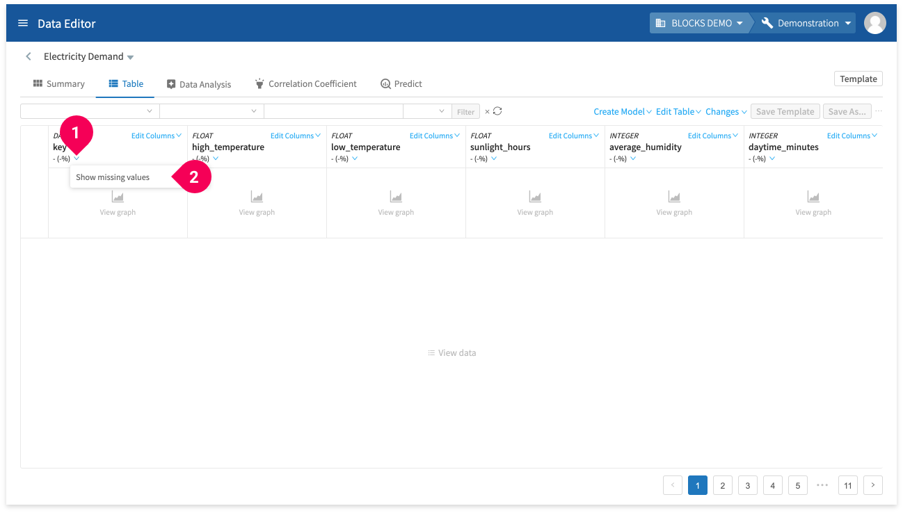
- Click keyboard_arrow_down.
- Click Show missing values.
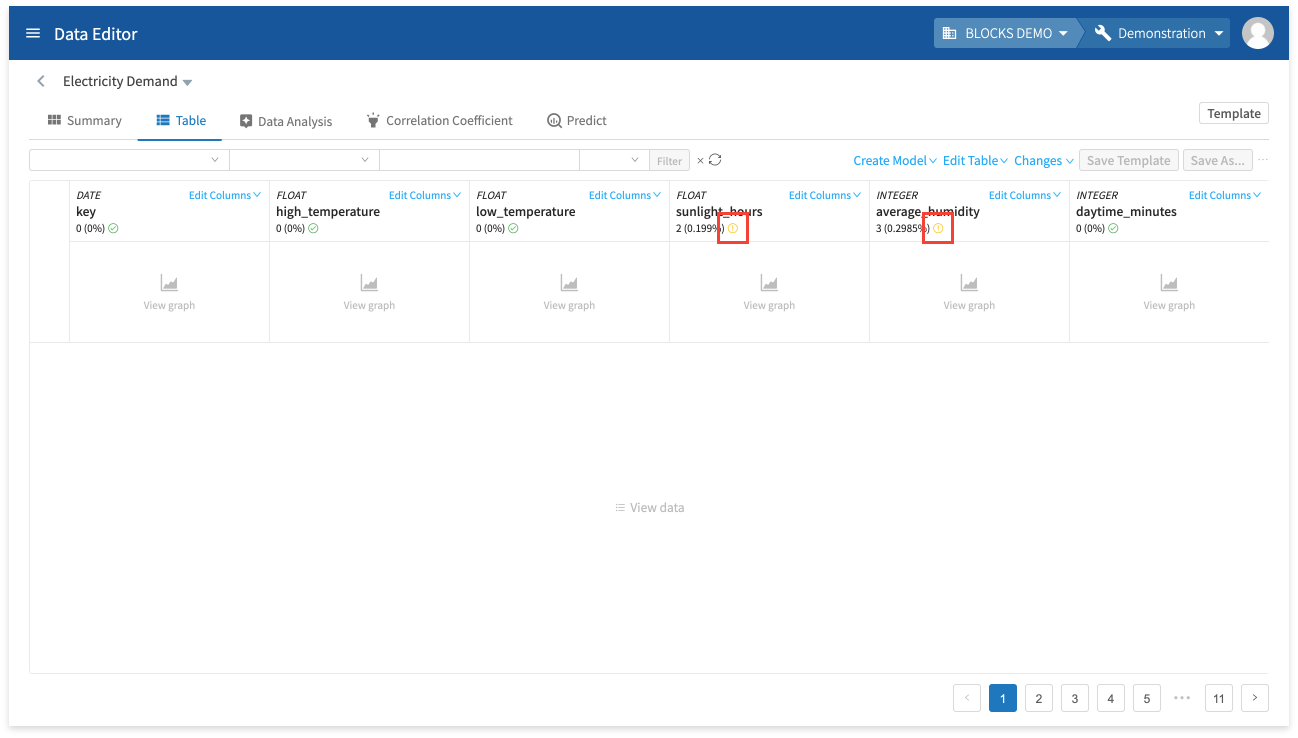
A error_outline will appear for any columns that contain missing values, as shown in the image above. For this data, the DataEditor will find missing values in the sunlight_hours and average_humidity columns.
We can’t use examples (rows) that contain missing values when training the model, so delete these rows by doing the following:
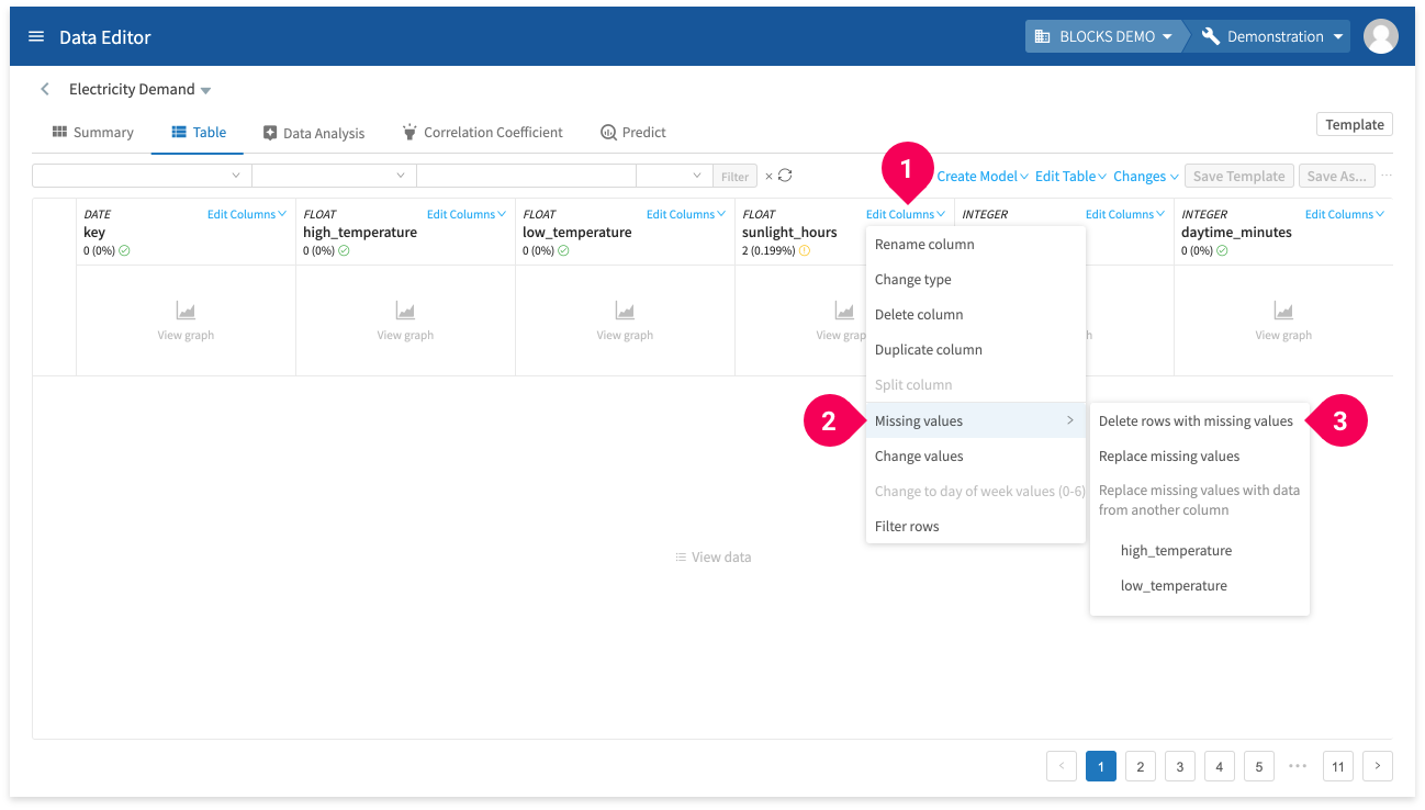
- Click Edit column.
- Click Missing values.
- Click Delete rows with missing values.
Repeat these steps for the average_humidity column.
The DataEditor keeps track of every edit that you make. You can view a list of these changes by doing the following:
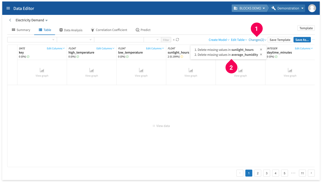
- Click Changes.
- Confirm that the list of changes contains the following:
- Delete missing values in sunlight_hours
- Delete missing values in average_humidity
info_outline You can click the × next to an item to revert that edit.
Save your changes by doing the following:
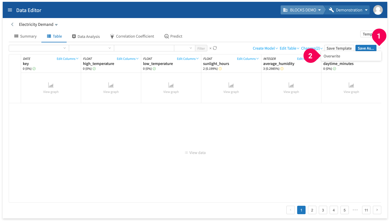
- Click more_horiz.
- Click Overwrite.
Not that you’ve cleansed the data of rows with missing values, split it into the training and testing data by doing the following:
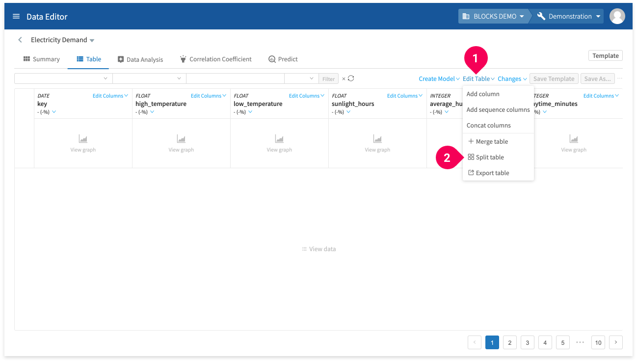
- Click Edit Table.
- Click Split table.
- Click Custom.
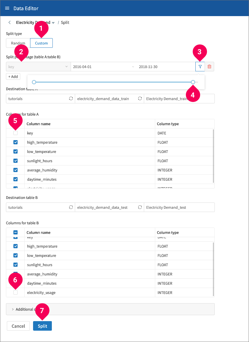
- Select key.
- Click the slider icon.
- Adjust the slider to the left until it shows 2018-11-30. You can also enter this date into the field directly.
- Uncheck key to remove the dates from the training data.
- Uncheck electricity_usage to remove the label column from the testing data.
- Click Split.
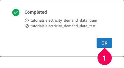
- Click OK.
The training and testing sets are organized as shown below:
In the following section, you’ll use the training data to train a regression model.
Training the model from the DataEditor
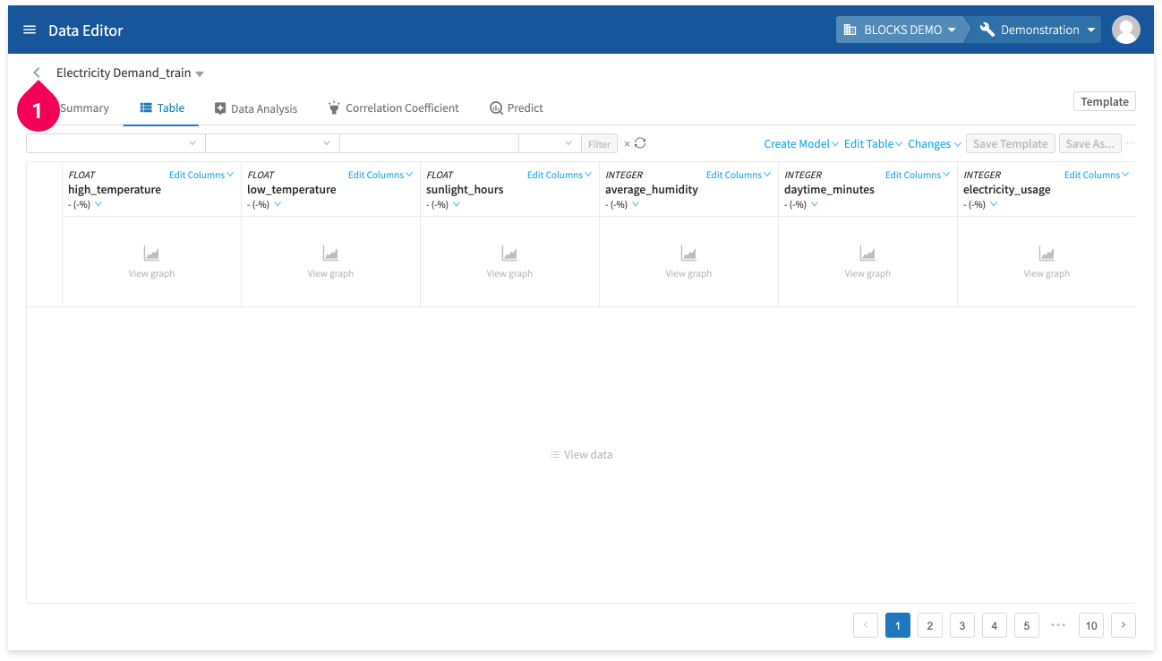
Use the training data you prepared to create a regression model by doing the following:
- Click Electricity Demand_train.
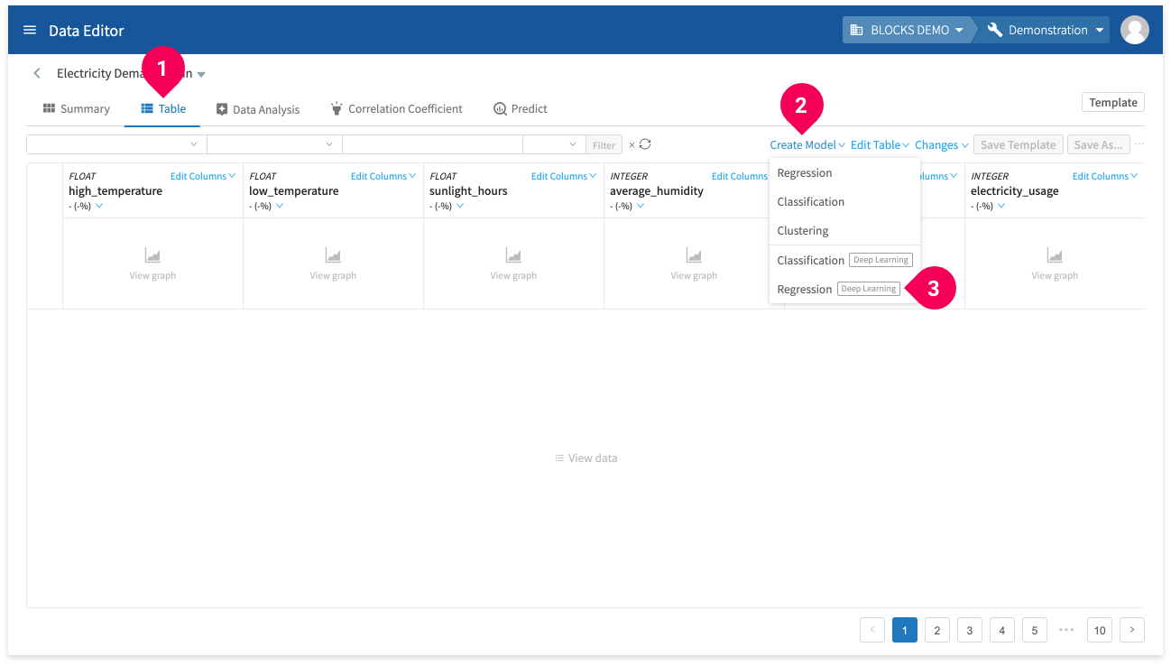
- If necessary, switch to the Table tab.
- Click Create Model.
- Click Regression (Deep Learning).
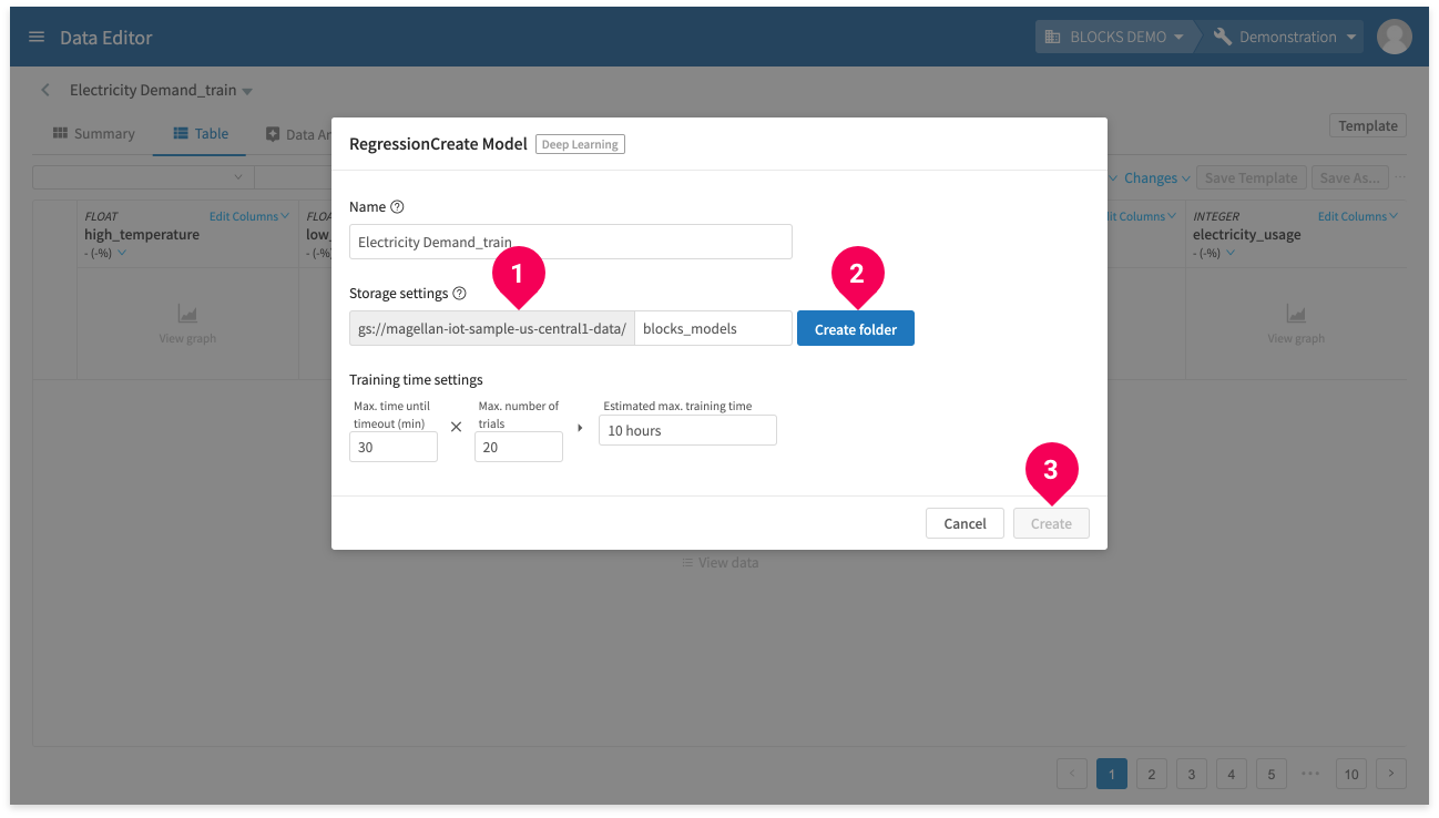
- Designate the Google Cloud Storage bucket (first time only).
- Enter the folder that will store your Deep Learning models and click Create Folder (first time only).
- Click Create.
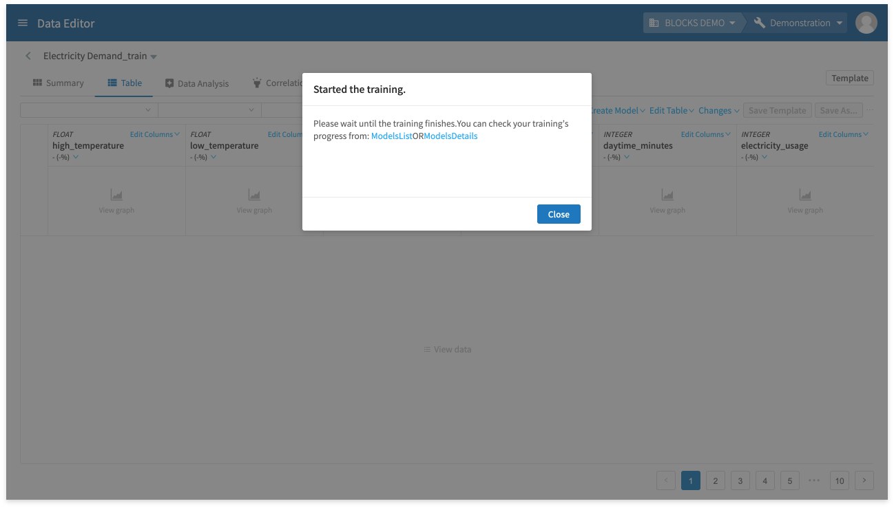
- Click Close.
Depending on server circumstances, it should take about 4–5 hours to train the model. You can check on the training’s progress from the model list or from the model’s details screen.
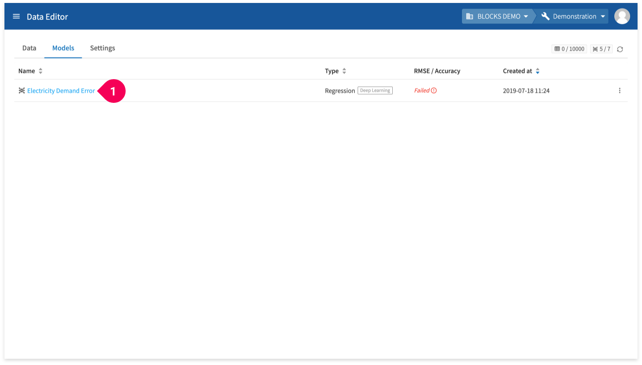
Switch to the model list by doing the following:
- Click <.
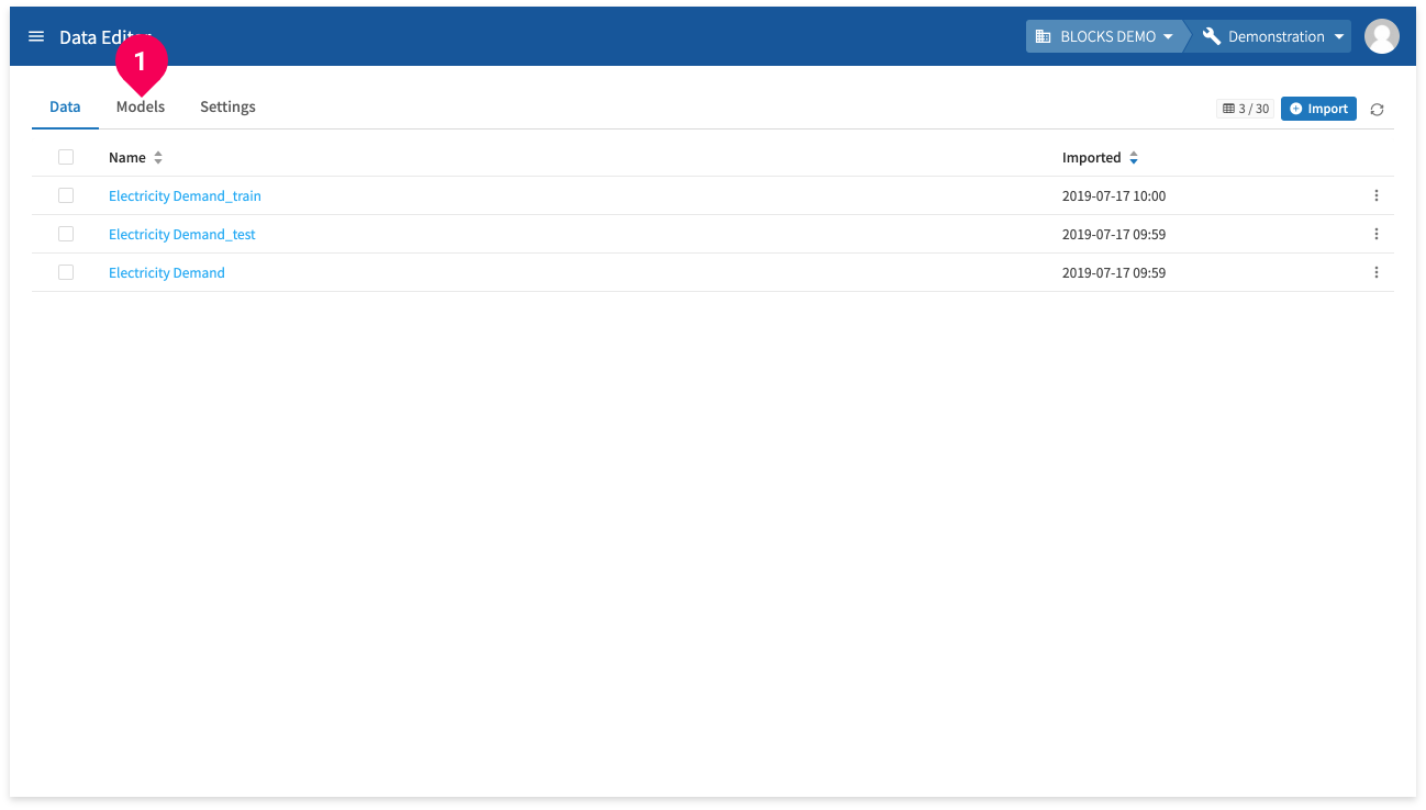
- Click Models.
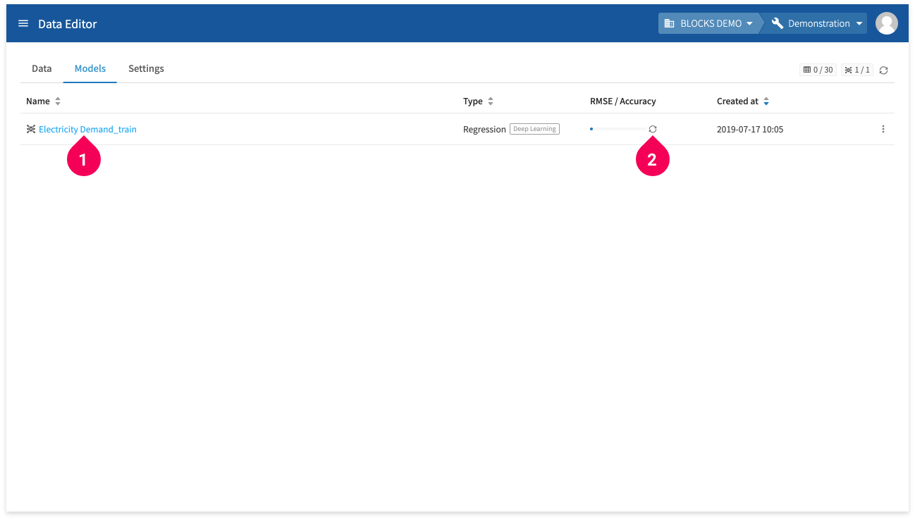
You can view a progress bar for the training in the RMSE/Accuracy column.
Clicking the training’s name (❶) will open its details page. You can also click the icon next to the progress bar (❷) to refresh it.
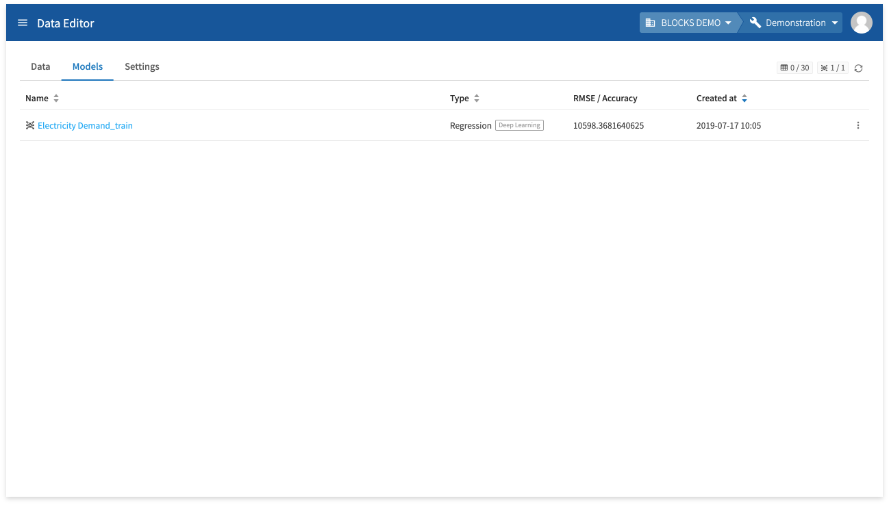
A value will appear in the RMSE/Accuracy column when the training finishes. In the next section, we’ll test the model by using it to make predictions in a Flow Designer.
Making predictions from a Flow Designer
This section will explain how to use a Flow Designer to make predictions.
You can also run predictions from the DataEditor, however it does not support batch predictions or setting automated schedules for running predictions like the Flow Designer does.
For more details on making predictions from the DataEditor, refer to Creating models and making predictions in the DataEditor.
Preparing a Flow Designer
In this section, we’ll use the Flow Templates feature in the Flow Designer to make predictions using the trained model. If you don’t have any Flow Designers yet, create one by doing the following:
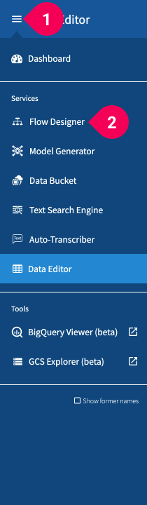
- Click the menu icon (menu) in the global navigation bar.
- Click Flow Designer.
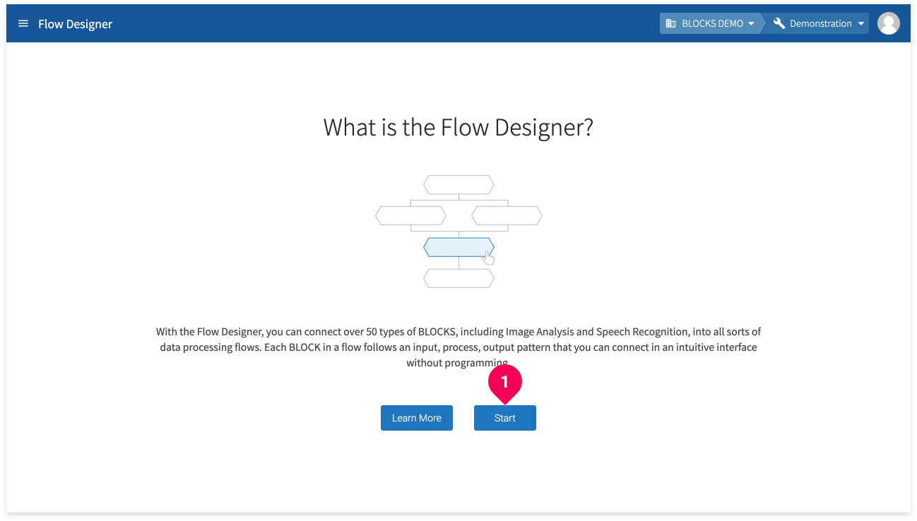
Click Start.
info_outline If you’ve already created a Flow Designer in your project, you’ll see the Flow Designer list instead of the page shown above. In this case, you can either use an existing Flow Designer or create a new one by clicking the “Add” button if you have sufficient licenses.
info_outline A message will appear if you don’t have enough licenses to create the Flow Designer. If you are an admin user in your organization, you’ll be given the option to purchase more licenses. Otherwise, you’ll be prompted to contact your organization’s admins.
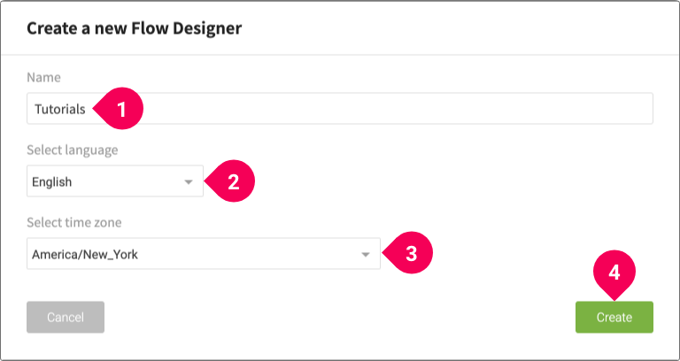
- Enter a name for the Flow Designer. We’ll use the name
Tutorials. - Select the language that will be used for log messages.
- Select your time zone.
- Click Create.
- Click the name of your Flow Designer from the list to open it in a new tab.
Creating a flow for predictions
In this section, you’ll create a processing flow that can make predictions with the trained model by doing the following:

- Click Flow Templates.
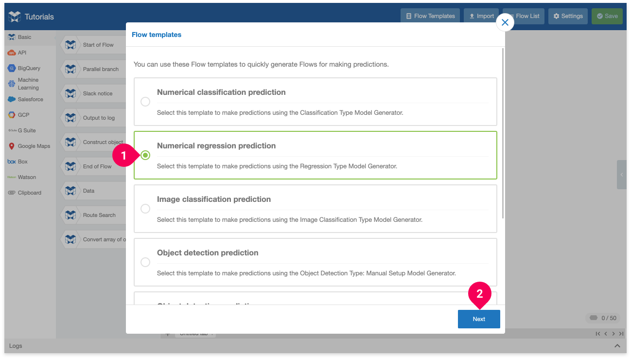
- Click Numerical regression.
- Click Next.
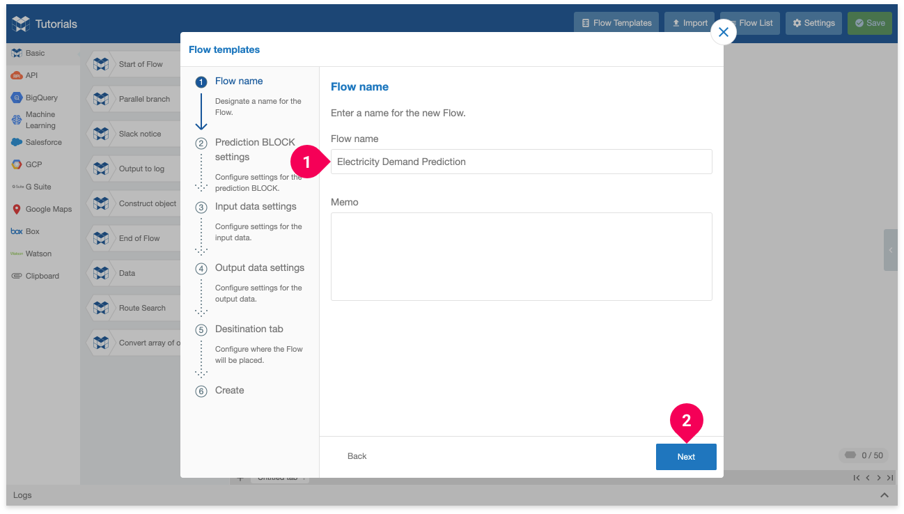
- Enter a name for the flow. We’ll use
Electricity Demand Prediction. - Click Next.
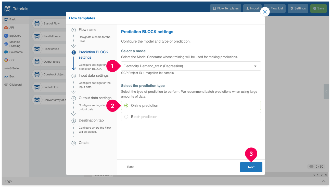
- Select the model you trained in the DataEditor. Ours is named Electricity Demand_train.
- Click Online prediction.
- Click Next.
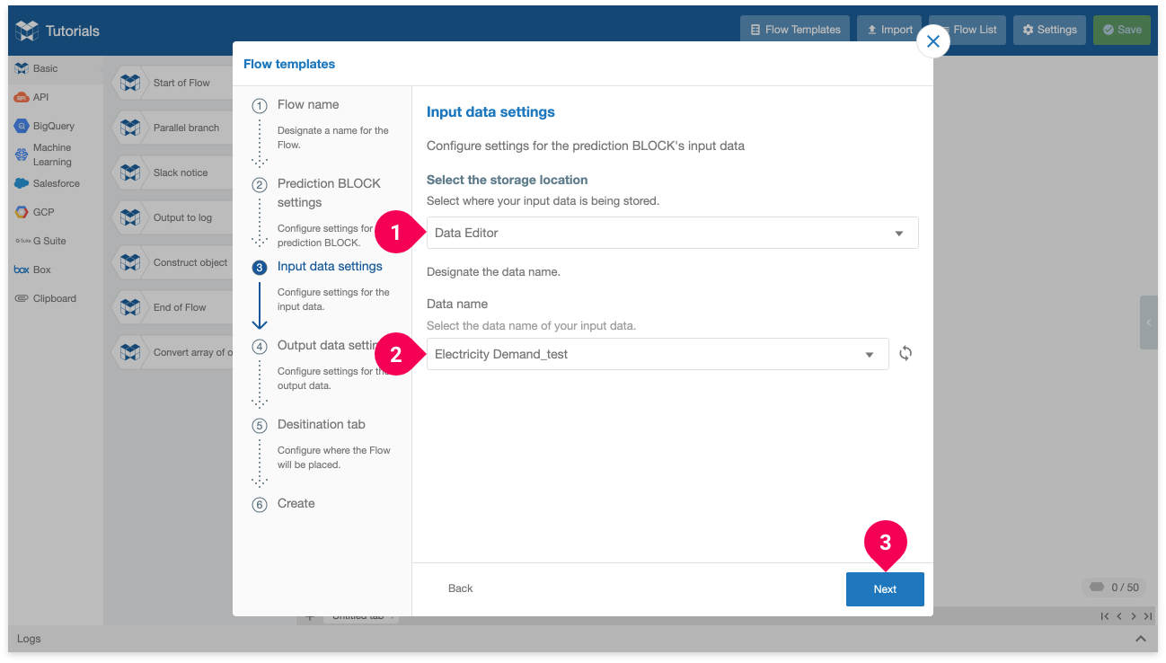
- Click DataEditor.
- Click the name of your test data. Ours is named Electricity Demand_test.
- Click Next.
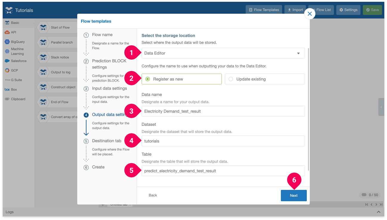
- Click DataEditor.
- Click Register as new.
- Enter the name that will be used to identify the results data in the DataEditor. We’ll use
Electricity Demand_test_result. - Enter the dataset that will store the results. We’ll use
tutorials. - Enter the table that will store the results. We’ll use
predict_electricity_demand_test_result. - Click Next.
This will output the results to the DataEditor as Electricity Demand_test_result.
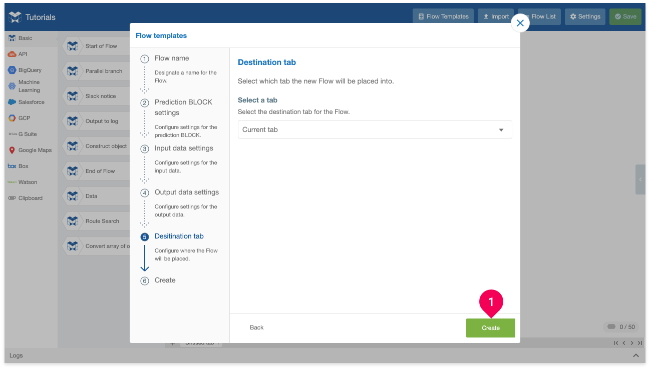
Click Create.
This will create the flow into your current tab in the Flow Designer. Save the new flow by doing the following:
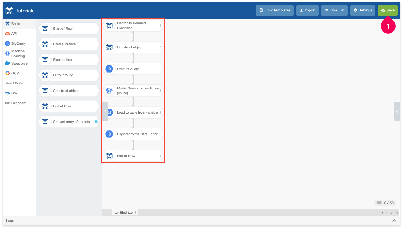
Click Save.
Executing the flow
With the Flow ready, you can execute it to make predictions by doing the following:
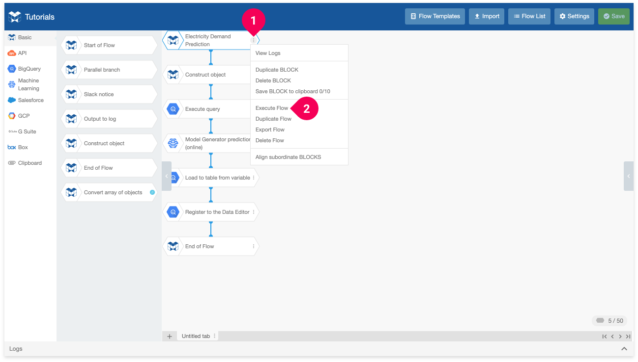
- Click the menu icon (more_vert) on the right side of the Electricity Demand Prediction (Start of flow) BLOCK.
- Click Execute Flow.
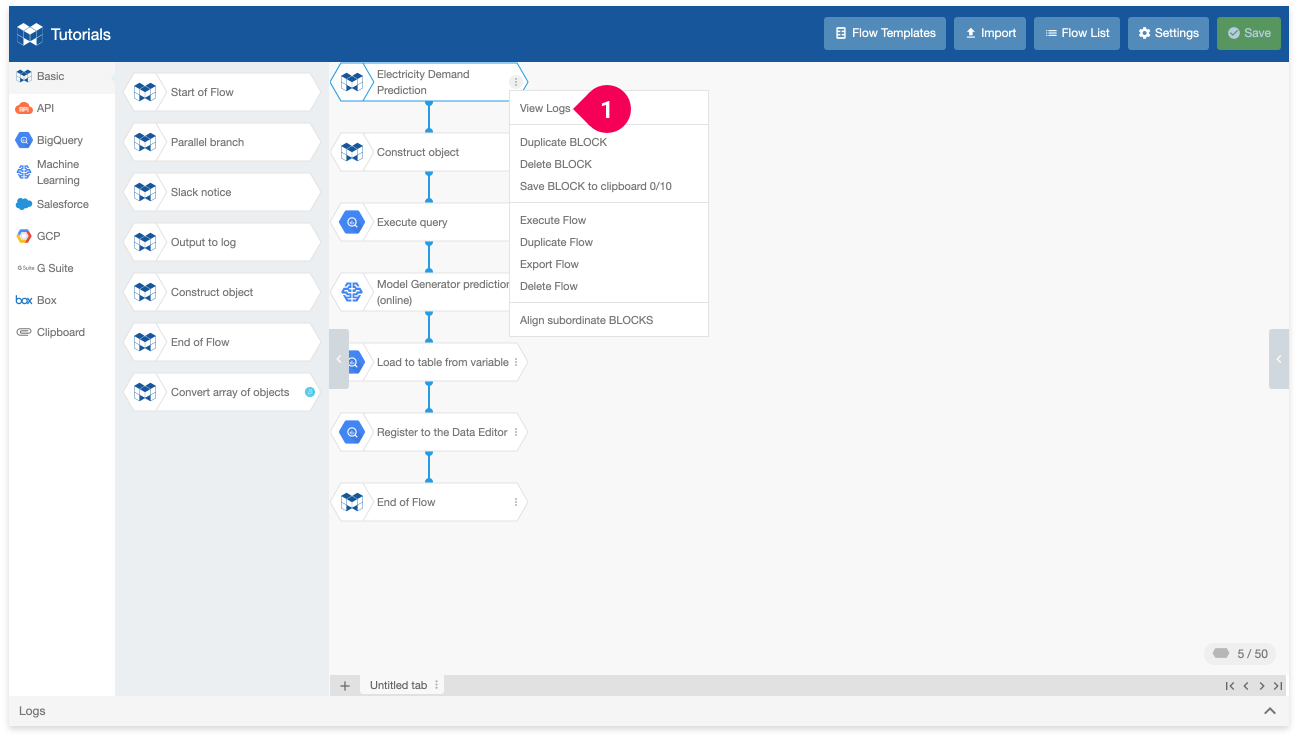
- Click View logs to open the logs panel and check the status of the flow while it executes.
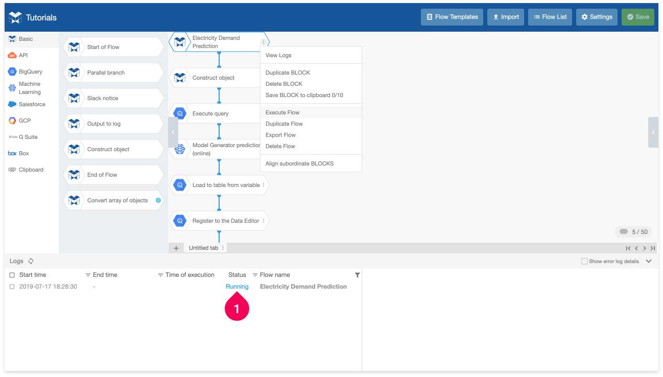
You can see the status of your Flow in the log list on the left side of the log panel. Its status will be Running (❶) while it executes. Wait for a bit of time until it finishes.
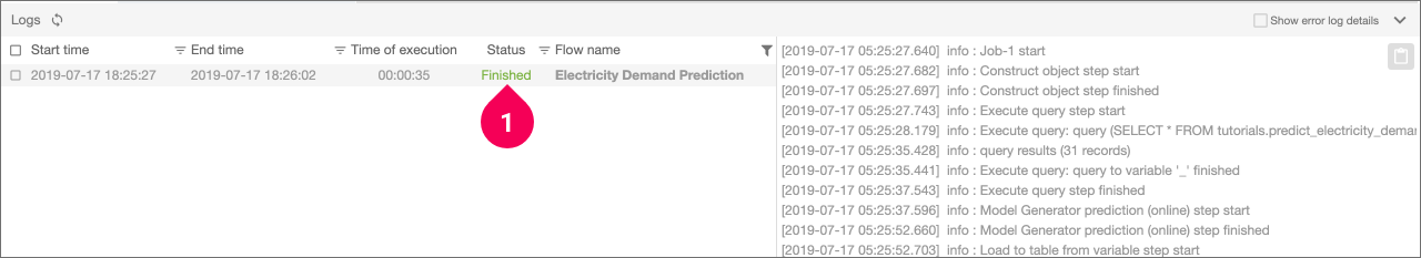
The status will change to a green Finished (❶) if the flow finishes executing successfully.
Checking the results in the DataEditor
The results of the prediction will be sent to the DataEditor, so return switch back to the BLOCKS tab and do the following:
- Click the menu icon (menu) in the global navigation bar.
- Click DataEditor.
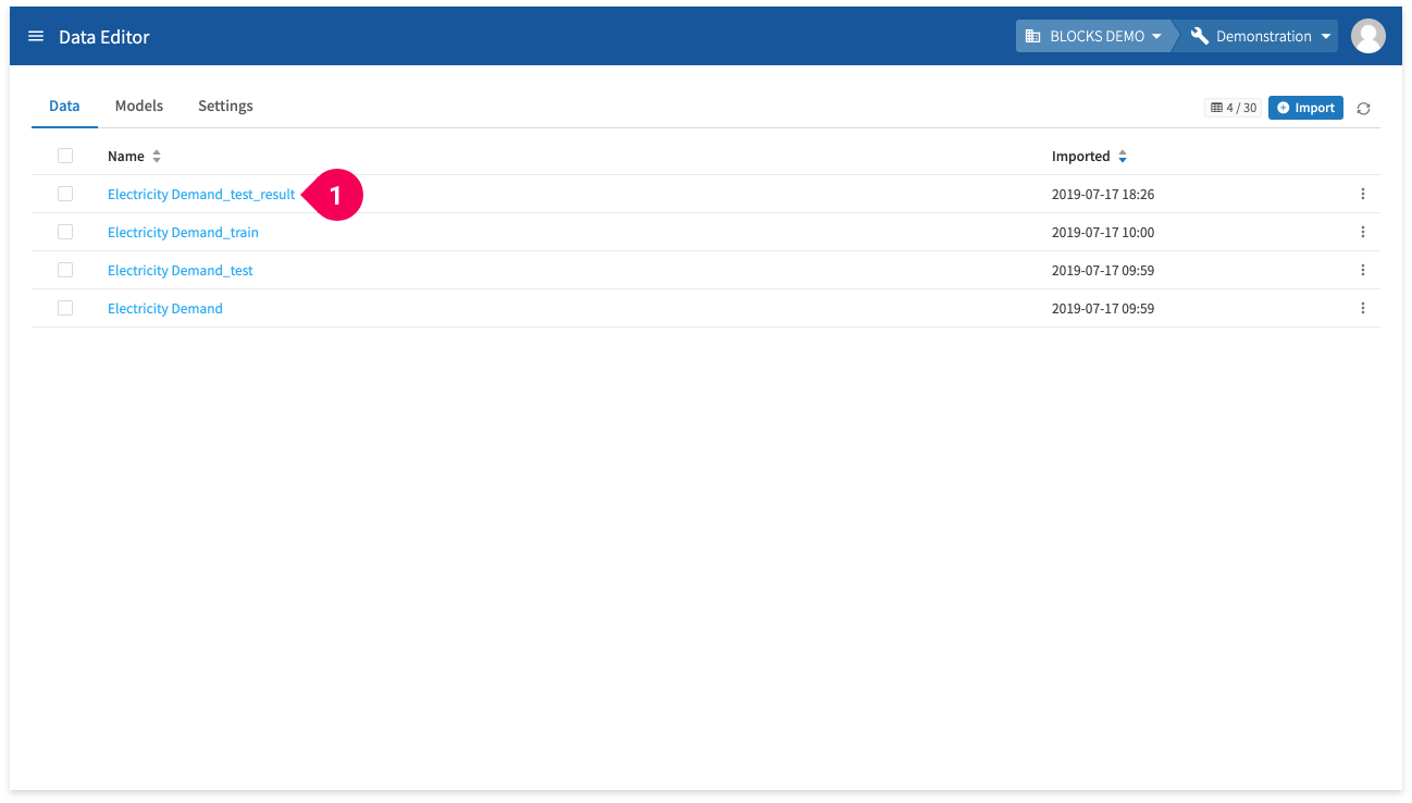
- Click the name for your results (you may need to click the reload button next to Import). Ours are Electricity Demand_test_result.
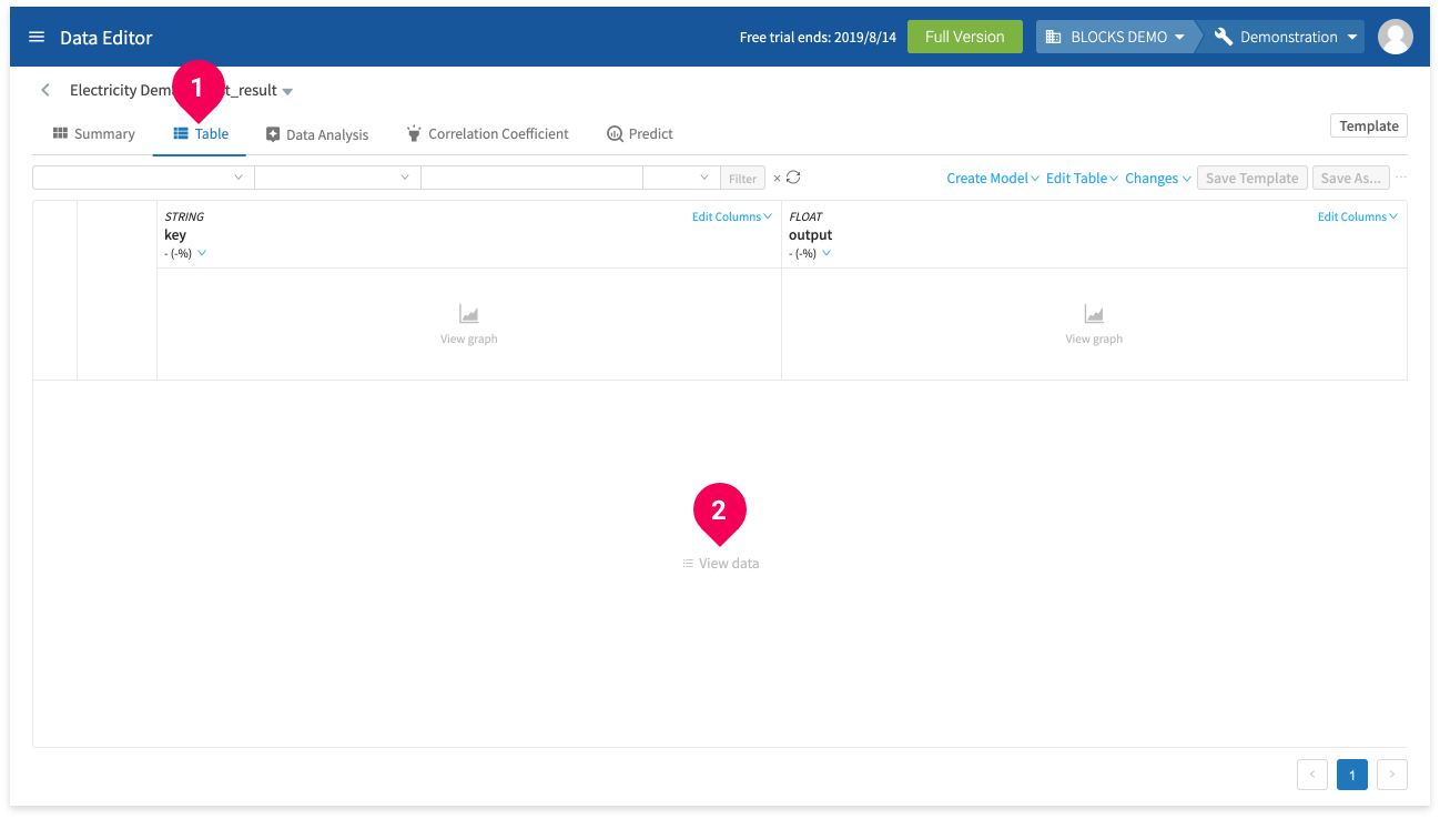
- Click Table.
- Click View data.
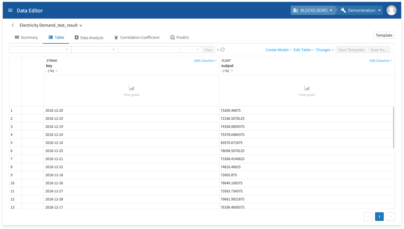
The following chart explains the meaning of each column:
| Name | Explanation |
|---|---|
| key |
The keys you configured for the prediction data. In this example, the keys are dates from 2018/12/1–2018/12/31. |
| output |
The value predicted for the corresponding key. In this example, this is the amount of electricity demand predicted for the corresponding date in the key column. |
We can now compare the predicted values with the actual electricity usage values for the same dates.
First, you’ll need to join the predicted and actual values into one table. To do this, you’ll need to convert the prediction result data’s key column from STRING to DATE type to match the initial data’s key column. To do this, do the following:
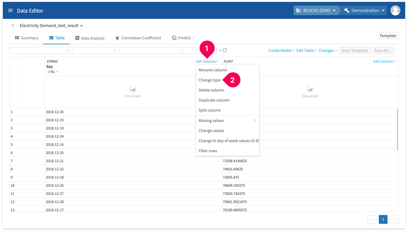
- Click Edit column for the key column.
- Click Change type.
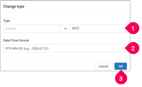
- Click DATE.
- Click YYYY-MM-DD.
- Click OK.
Save the changes by doing the following:
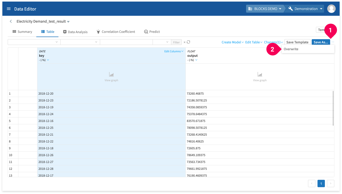
- Click more_horiz.
- Click Overwrite.
Join together this data with the actual electricity usage data by doing the following:
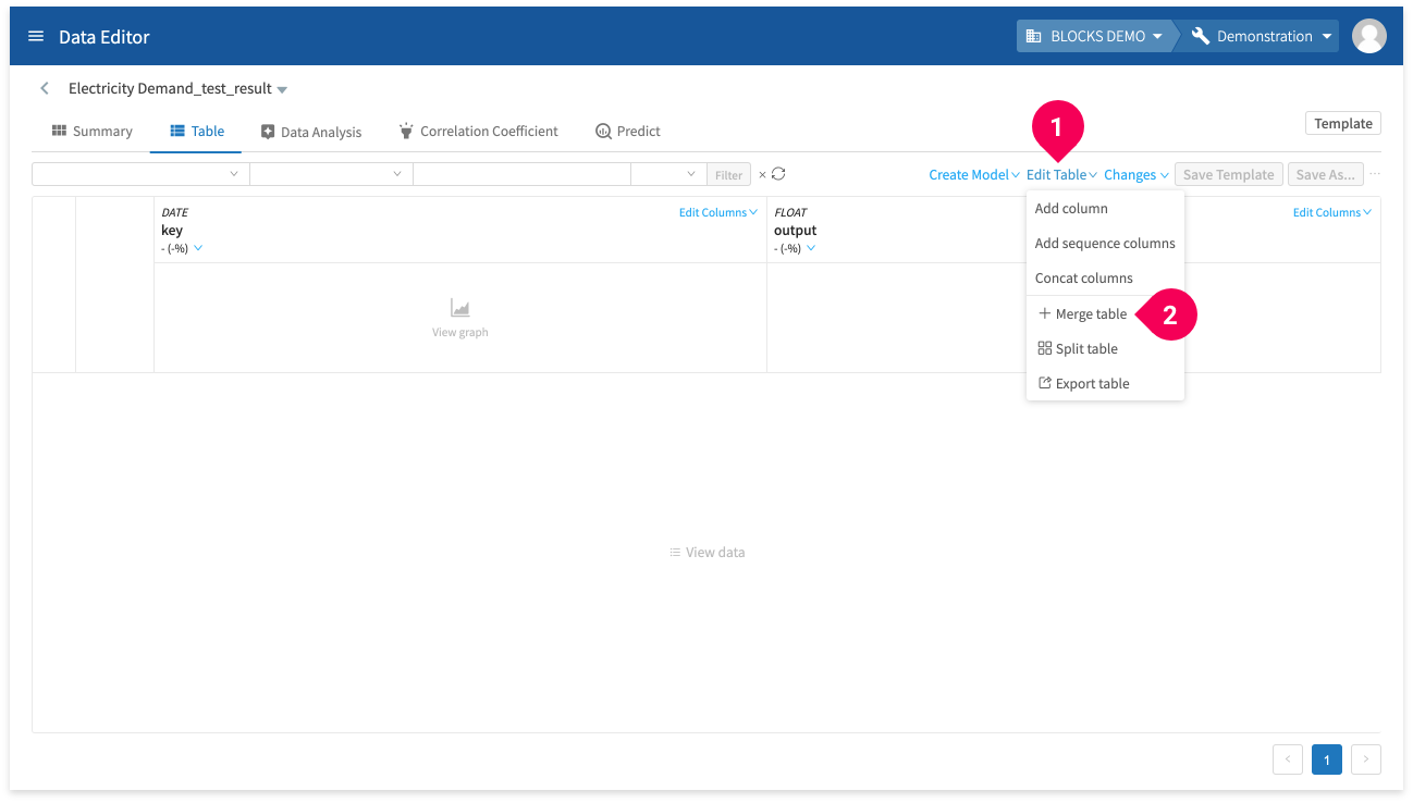
- Click Edit Table.
- Click Merge table.
Select to join this data with the actual electricity usage by doing the following:
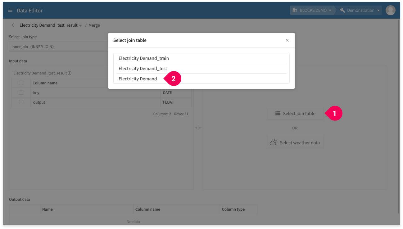
- Click Select Join Table.
- Click Electricity Demand.
Configure settings for how to join the data between the two tables by doing the following:
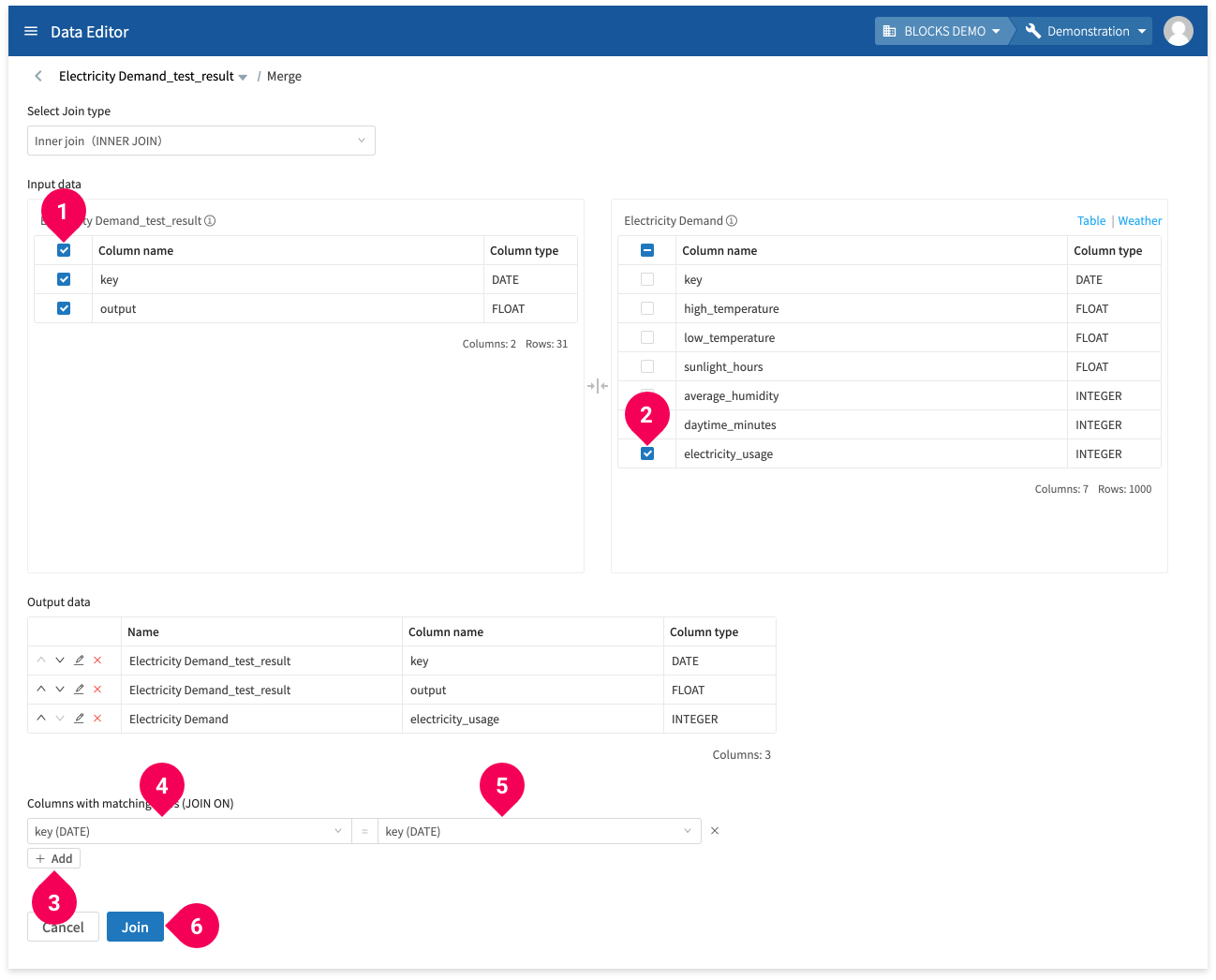
The join type should be set to Inner join (INNER JOIN) by default.
- Click the checkbox next to Column name to select all of the columns under Electricity Demand_test_result.
- Click the checkbox for electricity_usage under Electricity Demand.
- Click Add.
- Click key.
- Click key.
- Click Join.
Configure the location where the merged data will be stored by doing the following:
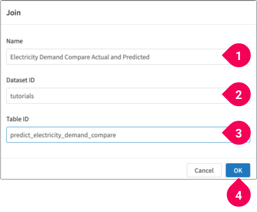
- Enter a name for the table. We’ll use
Electricity Demand Compare Actual and Predicted. - Select the dataset. We’ll use
tutorials. - Enter the table ID. We’ll use
predict_electricity_demand_compare. - Click OK.
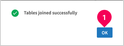
- Click OK.
Now that the data has been merged into one table, you can compare the actual and predicted electricity usage as a graph by doing the following:
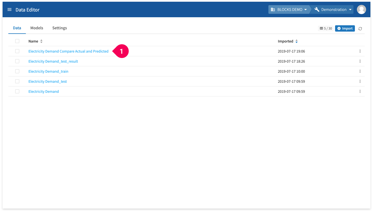
- Click Electricity Demand Compare Actual and Predicted.
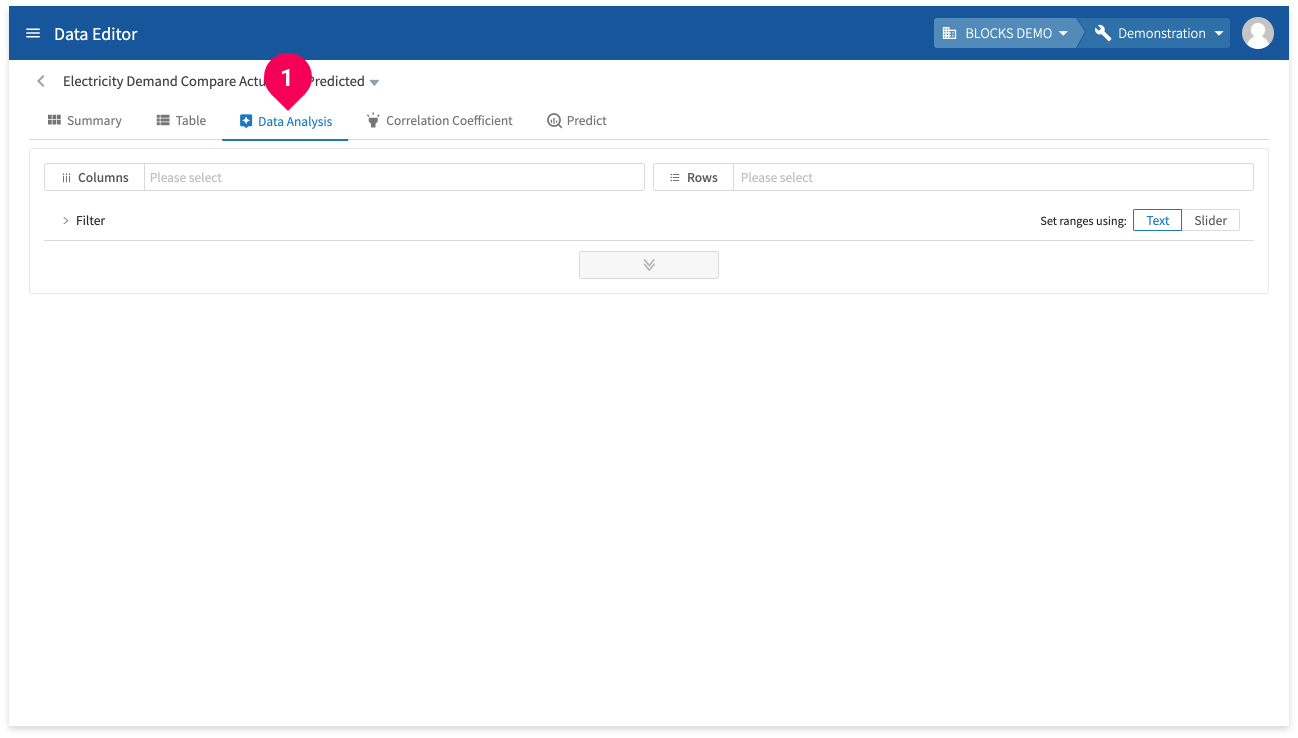
- Click Data Analysis.
Select the data to compare in the graph by doing the following:
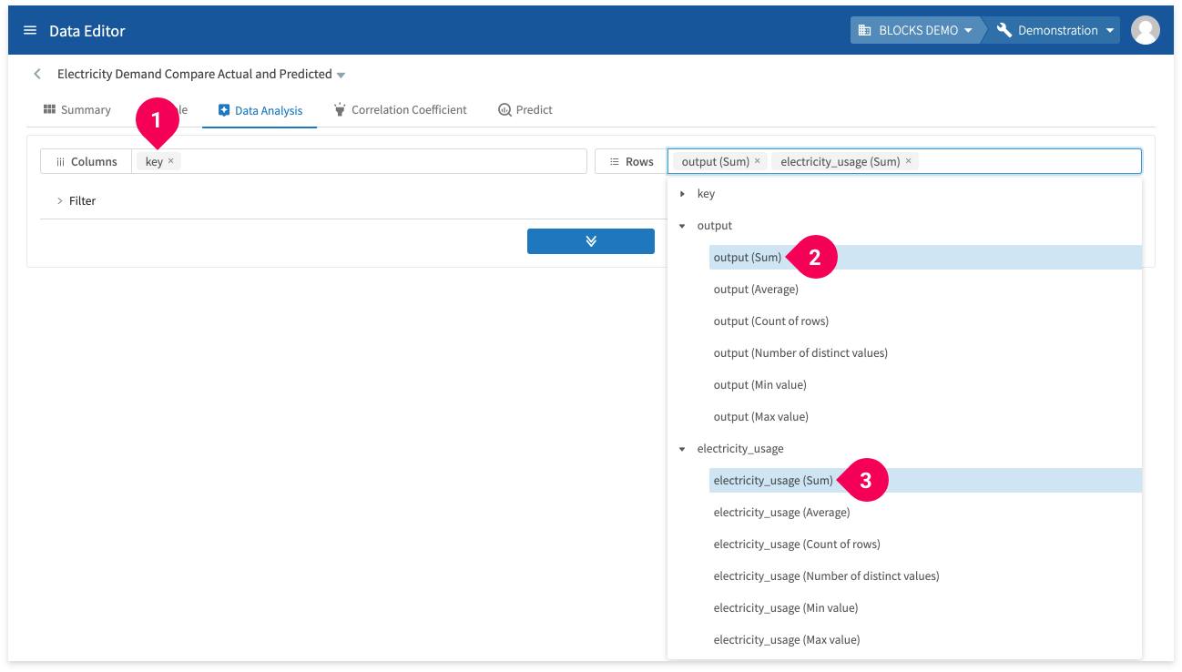
- For the columns field, select key.
- In the rows field, click to expand output and select output (Sum).
- In the rows field, click to expand electricity_usage and select electricity_usage (Sum).
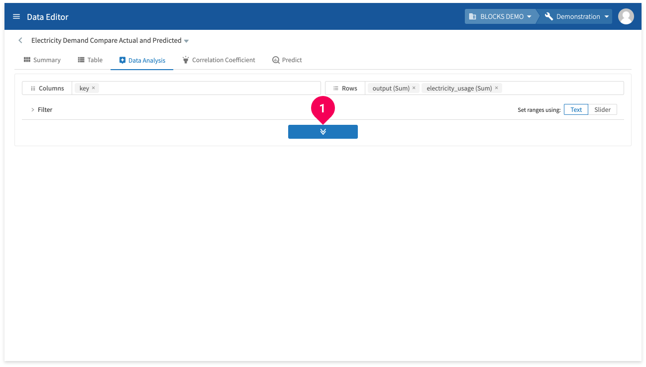
- Click the button in the center of the screen.
Switch to a line graph of the data by doing the following:
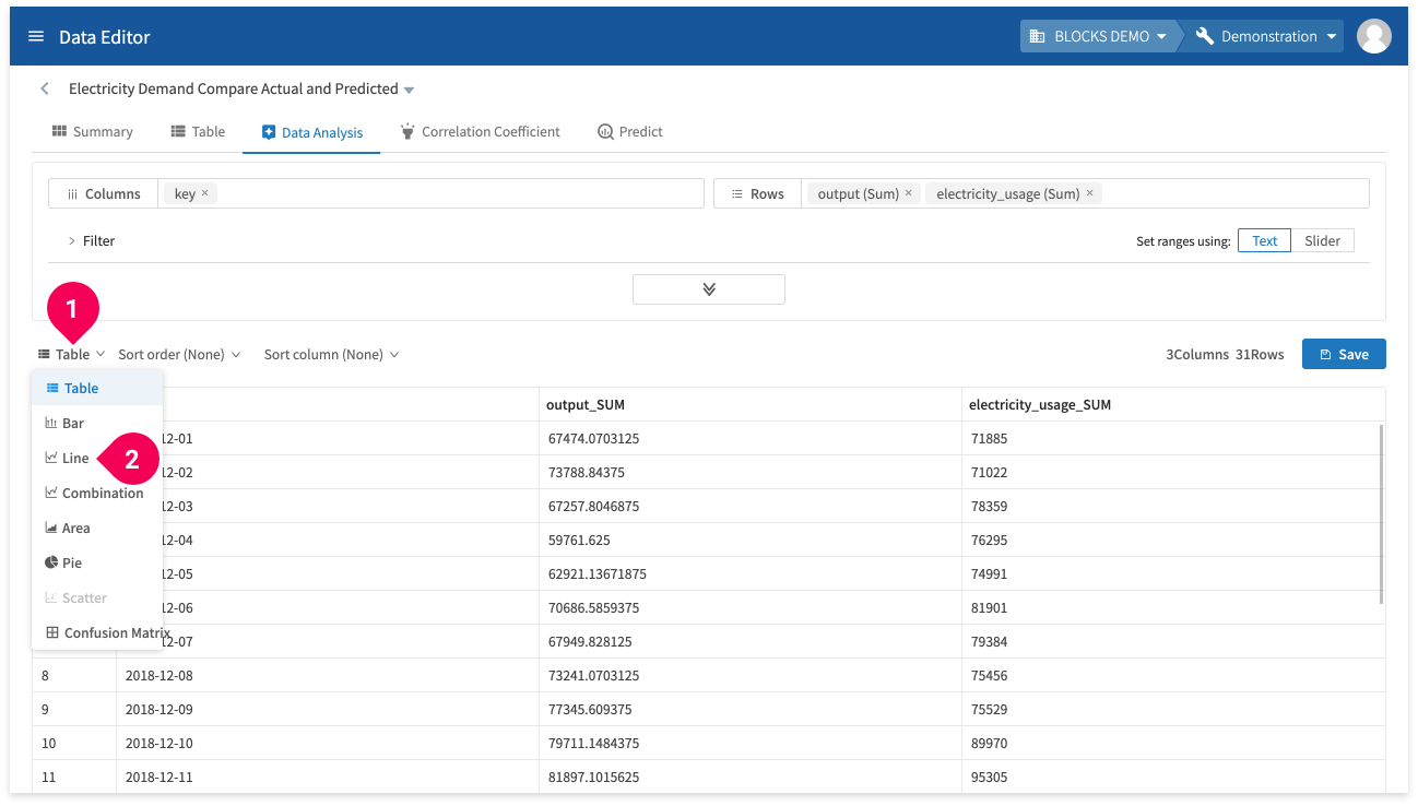
- Click Table.
- Click Line.
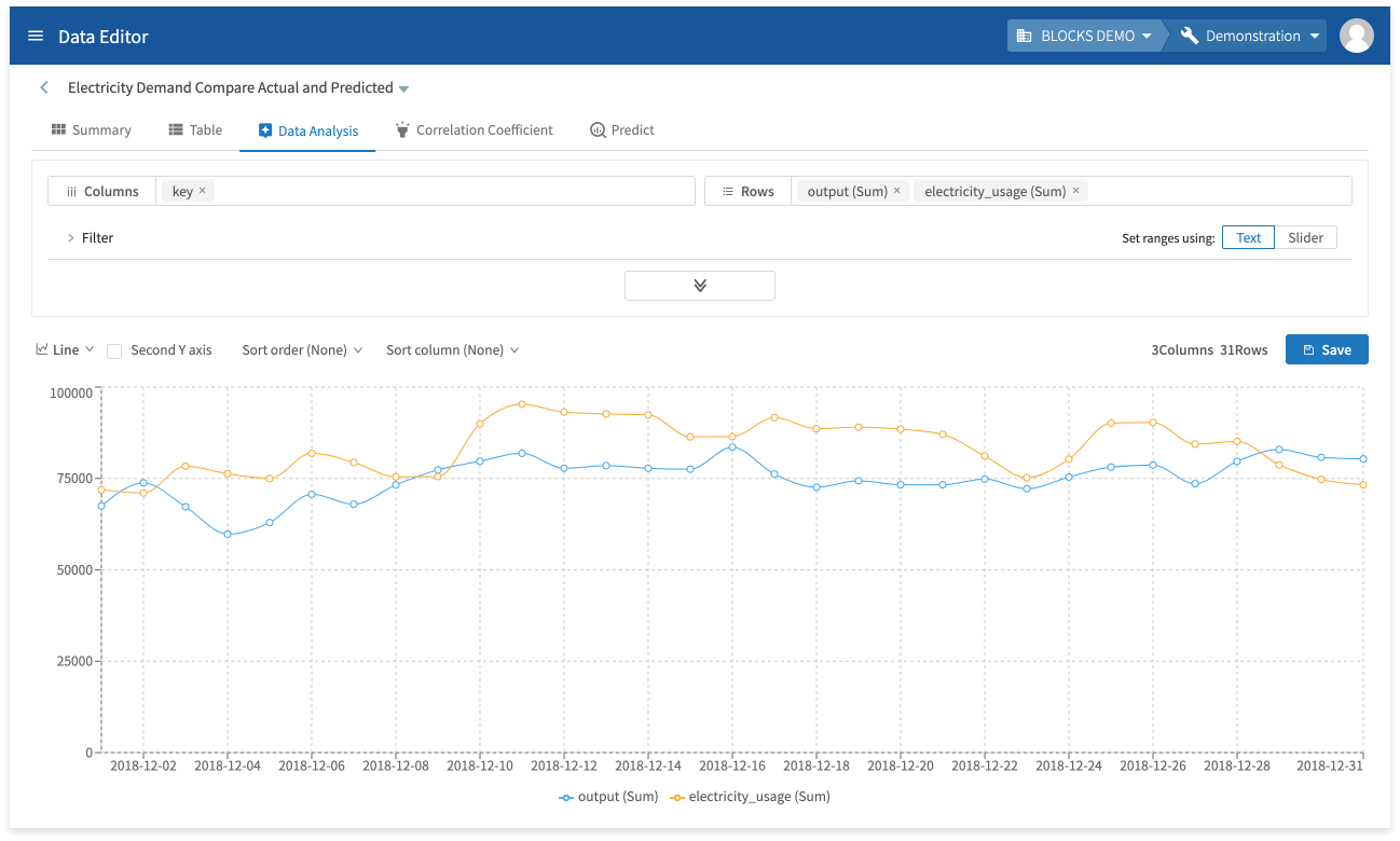
With a graph like this, you can easily compare the predicted and actual electricity usage and evaluate the effectiveness of your model.
However, judging whether or not your model is accurate enough depends on how you intend to use it. The example in this tutorial isn’t intended for any real use case, so we can’t say if it’s accurate enough or not. However, we will mention a few ways one could improve this model in the Summary section below.
With that, we’ve finished using BLOCKS to train a regression model, make predictions, and evaluate the results. We’ll explain what to do in case of errors in the following section.
In case of an error
If an error occurs during a training on the DataEditor, you can find the error logs by doing the following:
- Click the name of the model whose RMSE/Accuracy column shows Failed.
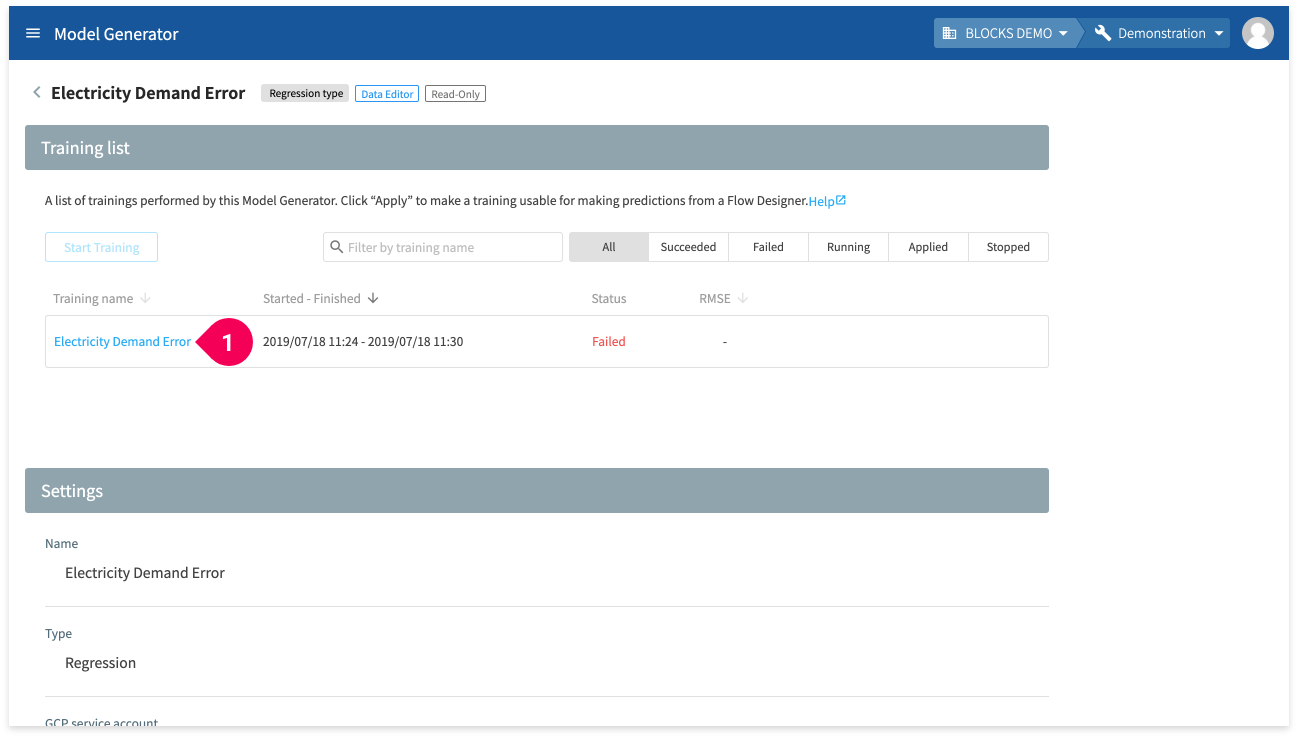
- Click the name of the training.
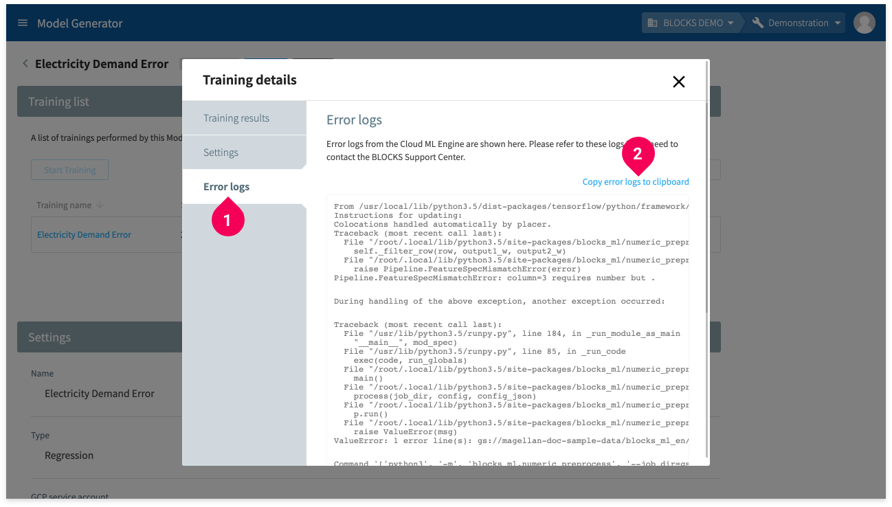
- Click Error logs.
- Click Copy error logs to clipboard.
If an error occurs on the Flow Designer, you can find the error logs in the logs panel. If you need to copy the error logs to contact BLOCKS Support, do the following:
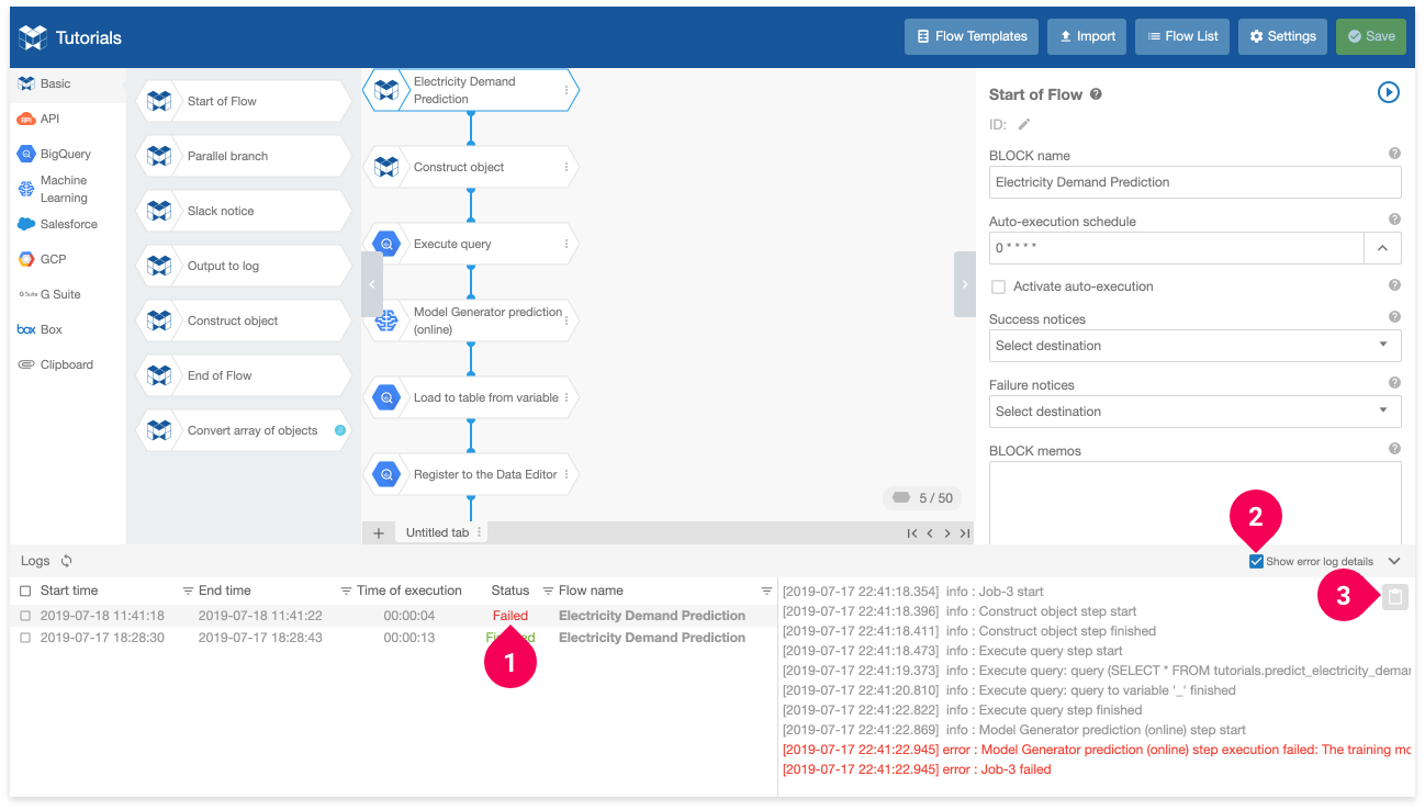
- Select the logs with the status Failed.
- Click Show error log details.
- Click the button to copy the logs.
Error messages in the Flow Designer are shown in red, but it’s often helpful to read the logs before and after the red error message.
If you encounter an error that you cannot solve after several attempts, you can contact the BLOCKS Support by clicking your user icon in the global navigation bar and selecting Contact Us. Please copy the entire contents of your error logs—not just the red lines—and include these either as a text file or within your message. For errors in a Flow Designer, you should also export your Flow as a JSON file and include this as an attachment in your message to BLOCKS support.
info_outline For more details on contacting BLOCKS Support, refer to the Basic Guide: Contact Us page.
Summary
With BLOCKS, training a regression model and making predictions doesn’t require specialized machine learning knowledge. All you need to do is prepare your data. However, there are a few points to keep in mind when doing this. In order to be usable by BLOCKS, your data should be a CSV file with UTF-8 encoding (without BOM).
While this tutorial doesn’t evaluate whether the trained model is accurate enough or not, it could certainly be improved by re-thinking the input features.
For example, there’s a strong possibility that electricity usage would be much lower on weekends and holidays when many companies are closed. You could try to improve on the model from this tutorial by adding features like the day of the week or whether or not it’s a holiday.
info_outline As with this tutorial, using machine learning to solve real business problems starts with gathering data. You may be able to use data your company already has, or you may need to take steps to gather or purchase new data. You then need to examine your data and determine which features to use, cleanse it of irregular values, and prepare it in the correct format for training a model. It's not an exaggeration to say that collecting and processing data makes up the better part of doing machine learning.